Download
1 / 29
320 likes | 547 Views
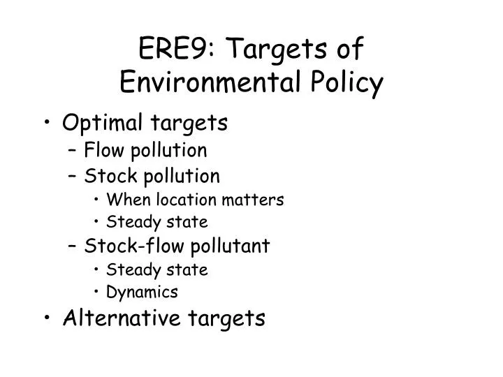
ERE9: Targets of Environmental Policy. Optimal targets Flow pollution Stock pollution When location matters Steady state Stock-flow pollutant Steady state Dynamics Alternative targets. Last week. Valuation theory Total economic value Indirect valuation methods Hedonic pricing

E N D
ERE9: Targets of Environmental Policy • Optimal targets • Flow pollution • Stock pollution • When location matters • Steady state • Stock-flow pollutant • Steady state • Dynamics • Alternative targets
Last week • Valuation theory • Total economic value • Indirect valuation methods • Hedonic pricing • Travel cost method • Direct valuation methods
Environmental & Resource Economics • Part 1: Introduction • Sustainability • Ethics • Efficiency and optimality • Part 2: Resource economics • Non-renewables • Renewables • Part 3: Environmental economics • Targets • Instruments • Part 4: Miscellaneous • Valuation (next course) • International environmental problems (next course) • Environmental accounting
Pollution • Pollution is an externality, that is, the unintended consequence of one‘s production or consumption on somebody else‘s production or consumption • Pollution damage depends on • Assimilative capacity of the environment • Existing loads • Location • Tastes and preferences of affected people • Pollution damage can be • Flow-damage pollution: D=D(M); M is the flow • Stock-damage pollution: D=D(A); A is the stock • Stock-flow-damage pollution: D=D(M,A)
Efficient Flow Pollution • Damages of pollution D=D(M) • Benefits of pollution B=B(M) • Net benefits NB=B(M)-D(M) • Efficient pollution Max NB
Efficient level of flow pollution emissions D(M) B(M) D(M) B(M) Total damage and benefit functions Maximised net benefits M * Marginal damage and benefit functions M* M
The economically efficient level of pollution minimises the sum of abatement and damage costs Costs, benefits Marginal benefit X Marginal damage Y A D C B M Quantity of pollution emission per period 0 M* M’
Types of externalities • Area B: Optimal level of externality • Area A+B: Optimal level of net private benefits of the polluter • Area A: Optimal level of net social benefits • Area C+D: Level of non-optimal externality that needs regulation • Area C: Level of net private benefits that are unwarranted • M*: Optimal level of economic activity • M‘: Level of economic activity that maximises private benefits
Efficient Flow Pollution (2) • Optimal pollution is greater than zero • The laws of thermodynamics imply that zero pollution implies zero activity, unless there are thresholds (e.g., assimilative capacity) • Optimal pollution is greater than the assimilative capacity • Pollution greater than the optimal pollution arises from discrepancies between social and private welfare
Stock pollutants lifetime Source: IPCC(WG1) 2001
Stock pollutants with short lifetime: When location matters Wind direction and velocity R1 R2 S1 S2 R4 R3 S: Source R: Urban area
Stock pollutants with longer lifetime: Efficient pollution • Damages of pollution • Benefits of pollution • Stock • Net current benefits • Efficient pollution Max NPVNB • Hamiltonian:
Steady State • Static efficiency • Dynamic efficiency • Steady state
Steady State (2) • Marginal benefit of the polluting activity equals the net present value of marginal pollution damages • Benefits of pollution are current only • Damages of pollution are a perpetual annuity • The decay rate ( ) acts as a discount rate
Steady State (3) Distinguish four cases:
Steady state: Case A • Case A • Equation collapses to • In the absence of discounting, an efficiency steady-state rate of emissions requires that • the marginal benefits of pollution should equal the marginal costs of the pollution flow • which equals the marginal costs of the pollution stock divided by its decay rate
Steady state: Case A (2) * M* M In the steady-state, A will have reached a level at which aA*=M*
Steady state: Cases A and B ** * M** M M* Case A: Case B:
Steady State: Cases C and D • Case C: • Case D: • The pollutant is perfectly persistent • In the absence of assimilation, the steady state can only be reached if emissions go to zero • Clean-up expenditures might allow for some positive level of emissions
Efficient Stock-Flow Pollution • Pollution flows are related to the extraction and use of a non-renewable resource • For example, brown coal (lignite) mining • What is the optimal path for the pollutant? • Two kind of trade offs • Intertemporal trade-off • More production generates more pollution • Pollution damages through • utility function • production function • E is an index for environmental pressure • V is defensive expenditure
The optimisation problem • Current value Hamiltonian: • Control variables: C, R, V • State variables: S, K, A • Co-state variables: P, w,l subject to
Shadow Price of Resource • Gross price = Net price + extraction costs + disutility of flow damage + loss of production due to flow damage + value of stock damage • Flow and stock damages need to be internalised!
Optimal time paths for the variables of the pollution model Pt+GR-UEER-QEER-MR Pt+GR-UEER-QEER Units of utility Pt+GR-UEER Stock damage Production flow damage Utility flow damage Pt+GR Gross price Marginal extraction cost Pt = net price Net price time, t
A competitive market economy where damage costs are internalised Units of utility Stock damage tax Pollution flow damage tax Utility damage tax Pt+GR= Gross price Social costs Marginal extraction cost Pt = net price Private costs Net price time, t
Efficient Clean-up • The shadow price of capital equals the shadow price of stock pollution times the marginal productivity of the clean-up activity • Ergo, environmental clean-up (defensive expenditure) is an investment like all other investments
Alternative Standards • Optimal pollution is but one way of setting environmental standards and not the most popular • The main difficulty lies in estimating the disutility of pollution • Alternatives • Arbitrary standards • Safe minimum standards • Best available technology (not exceeding excessive costs) • Precautionary principle