Download
1 / 37
370 likes | 581 Views
Hyperspectral Detection of Stressed Asphalt Meteo 597A Isaac Gerg. Fire Marshall Lampkin. Agenda. Overview of the Penn State Asphalt Laboratory Phenomenology Measuring asphalt spectra Laboratory findings Detection of asphalt targets in AVIRIS imagery Conclusion. Sample Asphalt Cores.

E N D
Hyperspectral Detection of Stressed AsphaltMeteo 597AIsaac Gerg
Agenda • Overview of the Penn State Asphalt Laboratory • Phenomenology • Measuring asphalt spectra • Laboratory findings • Detection of asphalt targets in AVIRIS imagery • Conclusion
“Baking” Pans Ovens
Lamp Optics Pi Pr Lambertian Surface Fiber Optic Cable
Radiometric Processor Optics
Calibration Spectrum Calibration Plate Nearly Flat Across All λ
The Samples M3273-SPT 12 Montour County M1BCBC MW 4.7 JB 4.2 M2288-SPT5 MD318 Td 25
Spectrum of Sample Sample
After Pouring Gasoline On Sample Dissolved Binder
Laboratory Findings • Fair amount of variability between the different asphalt cores we sampled • Not much variability between the treated cores • Very difficult to discriminate much less quantify • Asphalt should be burned longer • Burned for only 10-15 seconds • Didn’t notice any softening • Gasoline ran off top of sample and into pan • Need for experimentation in more realistic setting Modified data analysis to distinguish between types of asphalt
Detection Experiment • Hypothesis: It is possible to detect different asphalt types using hyperspectral imagery (HSI)? • Experiment • Measure spectra of different asphalt types in 400-2400nm range • Choose two target asphalt types to distinguish • Embed, at random pixel locations, several abundance amounts of target spectra into AVIRIS imagery using the 2005 AVIRIS noise model. Abundances used: [0.01:0.01:0.09 0.1:0.1:1.0] • Unmix image to recover endmembers • Use least squares techniques to measure abundance quantification • Repeat steps three to five 1000 times • Average results
Spectra of Targets Target 2 Target 1
Target 1 Detection Results nnlsMatlab ucls fclsMatlab fcls Error bars represent 95% confidence interval
Target 2 Detection Results nnlsMatlab ucls fclsMatlab fcls Error bars represent 95% confidence interval
Target 1 False Alarm Results ucls nnlsMatlab fclsMatlab fcls Target 1 detected when target 2 present
Target 2 False Alarm Results nnlsMatlab ucls fcls fclsMatlab Target 2 detected when target 1 present
Conclusions • Need to reevaluate experiment using more realistic conditions • Asphalt types are difficult to distinguish at pixel abundances less than 90% • Nonnegative least squares (NNLS) performed the best at abundance quantification when the target was actually present in the pixel • All of the constrained least squares methods outperformed the unconstrained least squares (UCLS) method regarding false detections (false alarms)
Thank You • Penn State Asphalt Laboratory • Dr. Solaimanian • Scott Milander • Dr. Lampkin • Provided portable radiometer • Dr. Kane • Dr. Fantle
Spectra of Targets Target 2 Target 1
Target 1 Detection Results nnlsMatlab ucls fclsMatlab fcls Only 100 trials conducted for these simulations
Target 2 Detection Results nnlsMatlab ucls fclsMatlab fcls Error bars represent 95% confidence interval
Target 1 False Alarm Results ucls nnlsMatlab fclsMatlab fcls Target 1 detected when target 2 present
Target 2 False Alarm Results nnlsMatlab ucls fcls fclsMatlab Target 2 detected when target 1 present