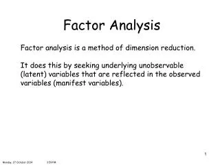
Factor Analysis Warning: Very Mathematical!

Factor Analysis Warning: Very Mathematical!

Motivating Example: McMaster’s Family Assessment Device • Consider the McMaster’s Family Assessment Device. It consists of 60 questions all on 4-point ordinal scale. • On some items a high score indicates good family functioning, while others are indicative of lower functioning. • Obviously many of the questions have some things in common and collectively measure different aspects of family functioning.

Motivating Example: McMaster’s Family Assessment Device (Q1-Q12) We can see the positive family traits measured by the even-numbered items and the negative family traits measured by the odd-numbered items are positively correlated amongst themselves and negatively correlated with each other as expected.

Motivating Example: McMaster’s Family Assessment Device But what does a subjects responses across all 12-items truly measure? We could simply add the items together, after reversing the scaling on the items that relate to the negative aspects of family functioning and family member interactions. After doing this a low total score would indicate a “good” family and a high total score would indicate a “bad” family. But perhaps there are different aspects of family functioning that the survey is measuring.

Factor Analysis • Factor analysis is used to illuminate the underlying dimensionality of a set of measures. • Some of these questions may cluster together to potentially measure things such things as communication, collaboration, closeness, or commitment. • This is the idea behind factor analysis.

Factor Analysis • Data reduction tool • Removes redundancy or duplication from a set of correlated variables. • Represents correlated variables with a smaller set of “derived” variables. These derived variables may measure some underlying features of the respondents. • Factors are formed that are relatively independent of one another. • Two types of “variables”: • latent variables: factors • observed variables (items on the survey)

Applications of Factor Analysis 1. Identification of Underlying Factors: • clusters variables into homogeneous sets • creates new variables (i.e. factors) • allows us to gain insight to categories 2. Screening of Variables: • identifies groupings to allow us to select one variable to represent many • useful in regression and other subsequent analyses

Applications of Factor Analysis 3. Summary: • flexibility in being able to extract few or many factors 4. Sampling of variables: • helps select small group of variables of representative yet uncorrelated variables from larger set to solve practical problem 5. Clustering of objects: • “inverse” factor analysis, we will see an example of this when examining a car model perception survey.

“Perhaps the most widely used (and misused) multivariate statistic is factor analysis. Few statisticians are neutral about this technique. Proponents feel that factor analysis is the greatest invention since the double bed, while its detractors feel it is a useless procedure that can be used to support nearly any desired interpretation of the data. The truth, as is usually the case,liessomewhere in between. Used properly, factor analysis can yield much useful information; when applied blindly, without regard for its limitations, it is about as useful and informative as Tarot cards. In particular, factor analysis can be used to explore the data for patterns, confirm our hypotheses, or reduce the many variables to a more manageable number.” -- Norman Streiner, PDQ Statistics

One Factor Model Classical Test Theory Idea: Ideal: X1 = F + e1 var(ej) = var(ek) , j ≠ k X2 = F + e2 … Xp= F + ep Reality: X1 = λ1F + e1 var(ej) ≠ var(ek) , j ≠ k X2 = λ2F + e2 … Xp= λpF + ep (unequal “sensitivity” to change in factor)

Key Concepts • F is latent (i.e. unobserved, underlying) variable called a factor. • X’s are the observed variables. • ejis measurement error for Xj. • λjis the “loading” on factor Ffor Xj.

Optional Assumptions • We will make these to simplify our discussions • X’s are standardized prior to beginning a factor analysis, i.e. converted to z-scores. • F is also standardized, that is the standard deviation of F is 1 and the mean is 0.

Some math associated with the ONE factor model • λj2 is also called the “communality” of Xj in the one factor case (Standard notation for communality: hj2) • For standardized Xj , Corr(F, Xj) = λj • For standardized variables, the percentage of variability in Xj explained by F is λj2. (like an R2 in regression) • If Xj is N(0,1) or at least standardized, then λj is equivalent to: • the slope in a regression of Xjon F • the correlation between F and Xj • Interpretation of λj: • standardized regression coefficient (regression) • path coefficient (path analysis) • factor loading (factor analysis)

Some moremath associated with the ONE factor model • Corr(Xj , Xk )= λjλk • Note that the correlation between Xj and Xk is completely determined by the common factor F. • Factor loadings (λj) are equivalent to correlation between factors and variables when only a SINGLE common factor is involved.

Example: McMaster’s FAD For the 12-items of McMaster’s FAD used in this survey we can see that the one factor solution essentially reverses the scales of the items measuring unhealthy family dynamics (-) and then “adds” up the items to get an overall score. The loadings are not all equal in magnitude so it does give more weight to some items than others.

Example: McMaster’s FAD The communalities ( are simply the squares of the factor loadings (. For example the communality for item 1 is: etc. This is one of the lowest communalities. We can also see that item 12 has the highest communality.

Steps in Exploratory Factor Analysis (EFA) (1) Collect data: choose relevant variables. (2) Extract initial factors (via principal components) (3) Choose number of factors to retain (4) Choose estimation method, estimate model (5) Rotate and interpret factors. (6) (a) Decide if changes need to be made (e.g. drop item(s), include item(s)) (b) repeat steps (4)-(5) (7) Construct scales or factor scores and potentially use them in further analysis. For example we might use the factor scores as predictors in a regression model for some response of interest.

Data Matrix • Factor analysis is totally dependent on correlations between variables. • Factor analysis summarizes correlation structure X1……...Xp F1…..Fm X1……...Xp X1 . . . Xp X1 . . . Xp O1 . . . . . . . . On ~ factor loadings Factor Matrix Correlation Matrix Data Matrix

Frailty Variables 12 tests yielding a numeric response Speed of fast walk (+) Upper extremity strength (+) Speed of usual walk (+) Pinch strength (+) Time to do chair stands (-) Grip strength (+) Arm circumference (+) Knee extension (+) Body mass index (+) Hip extension (+) Tricep skinfold thickness (+) Time to do Pegboard test (-) Shoulder rotation (+)

Frailty Example (n = 571) | arm ski fastw grip pincrupex knee hipextshldr peg bmiusalk ---------+------------------------------------------------------------------------------------ skinfld | 0.71 | | | | | | | | | | | fastwalk | -0.01 0.13 | | | | | | | | | | gripstr | 0.34 0.26 0.18 | | | | | | | | | pinchstr | 0.340.33 0.16 0.62 | | | | | | | | upextstr | 0.12 0.14 0.26 0.31 0.25 | | | | | | | kneeext | 0.16 0.310.35 0.28 0.28 0.21 | | | | | | hipext | 0.11 0.28 0.18 0.24 0.24 0.15 0.56 | | | | | shldrrot | 0.03 0.11 0.25 0.18 0.19 0.36 0.30 0.17 | | | | pegbrd | -0.10 -0.17 -0.34 -0.26 -0.13 -0.21 -0.15 -0.11 -0.15 | | | bmi | 0.880.64 -0.09 0.25 0.28 0.08 0.13 0.13 0.01 -0.04 | | uslwalk | -0.03 0.09 0.89 0.16 0.13 0.27 0.30 0.14 0.22 -0.31 -0.10 | chrstand | 0.01 -0.09 -0.43 -0.12 -0.12 -0.22 -0.27 -0.15 -0.09 0.25 0.03 -0.42

More than One Factor • m factor orthogonal model • ORTHOGONAL = INDEPENDENT, meaning the underlying factors F1, …, Fmare uncorrelated. • m factors, pobserved variables X1= λ11F1 + λ12F2 +…+ λ1mFm + e1 X2 = λ21F1 + λ22F2 +…+ λ2mFm + e2 ……. Xp= λp1F1+ λp2F2+…+ λpmFm+ ep

More than One Factor • Same general assumptions as one factor model. • Corr(Fs,Xj) = λjs • Plus: - Corr(Fs,Fr) = 0 for all s ≠ r (i.e. orthogonal) - this is forced independence - simplifies covariance/correlation structure - Corr(Xi,Xj) = λi1 λj1+ λi2 λj2+ λi3 λj3+….

Factor Matrix • Columns represent derived factors • Rows represent input variables • Loadings represent degree to which each of the variables “correlates” with each of the factors • Loadings range from -1 to 1 • Inspection of factor loadings reveals extent to which each of the variables contributes to the meaning of each of the factors. • High loadings provide meaning and interpretation of factors (~ regression coefficients) Ex: Car Rating Survey

Frailty Variables Speed of fast walk (+) Upper extremity strength (+) Speed of usual walk (+) Pinch strength (+) Time to do chair stands (-) Grip strength (+) Arm circumference (+) Knee extension (+) Body mass index (+) Hip extension (+) Tricep skinfold thickness (+) Time to do Pegboard test (-) Shoulder rotation (+)

Communalities • The communality of Xj is the proportion of the variance of Xj explained by the m common factors: • Recall one factor model:What was the interpretation of λj2? • In other words, it can be thought of as the sum of squared multiple-correlation coefficients between the Xj and the factors. • Uniqueness(Xj) = 1 - Comm(Xj)

Communality of Xj “Common” part of variance - correlation between Xj and the part of Xj due to the underlying factors, assuming Xjis standardized. - Var(Xj) = “communality” +”uniqueness” - For standardized Xj: 1 = “communality” +”uniqueness” - Thus, Uniqueness = 1 – Communality - Can think of Uniqueness = Var(ej)  If Xj is informative, communality is high  If Xj is not informative, uniqueness is high Intuitively: variables with high communality share more in common with the rest of the variables.

How many factors? Intuitively: The number of uncorrelated constructs that are jointly measured by the X’s. Factor analysis is only useful if number of factors is less than number of X’s. Requires decent correlation structure in the X’s.(Goal: “data reduction”) Identifiability: Is there enough information in the data to estimate all of the parameters in the factor analysis? May be constrained to a certain number of factors. Generally we like to have 10 observations per X in order to estimate underlying.

Choosing Number of Factors Use “principal components” to help decide • type of factor analysis (PCA) • number of factors is equivalent to number of variables • each factor is a weighted combination of the input variables: F1 = a1X1 + a2X2 + …. • Recall: For a factor analysis, generally, X1 = a1F1 + a2F2 +...

Estimating Principal Components • The first PC is the linear combination with maximum variance, • That is, it finds to maximize Var(F1) = constrained such that • First PC: linear combination that maximizes Var(a1TX) such that • Second PC: Linear combinationthat maximizes Var(a2TX) such that AND Corr(F1,F2)=0 • And so on…..

Eigenvalues • We use eigenvalues to select how many factors to retain. • We usually consider the eigenvalues from a principal components analysis (PCA). • Two interpretations: • eigenvalue  equivalent number of variables which the factor represents • eigenvalue  amount of “variance” in the data described by the factor. • Rules to go by: • number of eigenvalues > 1 • scree plot • % variance explained • comprehensibility

Frailty Example (p = 13) PCA = principal components; all p = 13 components retained Component Eigenvalue Difference Proportion Cumulative ------------------------------------------------------------------ 1 3.80792 1.28489 0.2929 0.2929 2 2.52303 1.28633 0.1941 0.4870 3 1.23669 0.10300 0.0951 0.5821 4 1.13370 0.19964 0.0872 0.6693 5 0.93406 0.15572 0.0719 0.7412 6 0.77834 0.05959 0.0599 0.8011 7 0.71875 0.13765 0.0553 0.8563 8 0.58110 0.18244 0.0447 0.9010 9 0.39866 0.02716 0.0307 0.9317 10 0.37149 0.06131 0.0286 0.9603 11 0.31018 0.19962 0.0239 0.9841 12 0.11056 0.01504 0.0085 0.9927 13 0.09552 . 0.0073 1.0000

Scree Plot for Frailty Example

First 6 Factors from PCA PCA Factor Loadings Variable | 1 2 3 4 5 6 ----------+----------------------------------------------------------------- arm_circ | 0.28486 0.44788 -0.26770 -0.00884 0.11395 0.06012 skinfld | 0.32495 0.31889 -0.20402 0.19147 0.13642 -0.03465 fastwalk | 0.29734 -0.39078 -0.30053 0.05651 0.01173 0.26724 gripstr | 0.32295 0.08761 0.24818 -0.37992 -0.41679 0.05057 pinchstr | 0.31598 0.12799 0.27284 -0.29200 -0.38819 0.27536 upextstr | 0.25737 -0.11702 0.17057 -0.38920 0.37099 -0.03115 kneeext | 0.32585 -0.09121 0.30073 0.45229 0.00941 -0.02102 hipext | 0.26007 -0.01740 0.39827 0.52709 -0.11473 -0.20850 shldrrot | 0.21372 -0.14109 0.33434 -0.16968 0.65061 -0.01115 pegbrd | -0.22909 0.15047 0.22396 0.23034 0.11674 0.84094 bmi | 0.24306 0.47156 -0.24395 0.04826 0.14009 0.02907 uslwalk | 0.27617 -0.40093 -0.32341 0.02945 0.01188 0.29727 chrstand | -0.21713 0.27013 0.23698 -0.10748 0.19050 0.06312

At this stage…. • Don’t worry about interpretation of factors! • Main concern: whether a smaller number of factors can account for variability • Researcher (i.e. YOU) needs to: • provide number of common factors to be extracted OR • provide objective criterion for choosing number of factors (e.g. scree plot, % variability, etc.)

Rotation • In principal components, the first factor describes most of variability. • After choosing number of factors to retain, we want to spread variability more evenly among factors. • To do this we “rotate” factors: • redefine factors such that loadings on various factors tend to be very high (-1 or 1) or very low (0) • intuitively, this makes sharper distinctions in the meanings of the factors • We use “factor analysis” for rotation NOT principal components!

5 Factors, Unrotated PCA Factor Loadings Variable | 1 2 3 4 5 Uniqueness ----------+----------------------------------------------------------------- arm_circ | 0.59934 0.67427 -0.26580 -0.04146 0.02383 0.11321 skinfld | 0.62122 0.41768 -0.13568 0.16493 0.01069 0.39391 fastwalk | 0.57983 -0.64697-0.30834 -0.00134 -0.05584 0.14705 gripstr | 0.57362 0.08508 0.31497-0.33229 -0.13918 0.43473 pinchstr | 0.55884 0.13477 0.30612 -0.25698 -0.15520 0.48570 upextstr | 0.41860 -0.15413 0.14411 -0.17610 0.26851 0.67714 kneeext | 0.56905 -0.14977 0.26877 0.36304 -0.01108 0.44959 hipext | 0.44167 -0.04549 0.315900.37823 -0.07072 0.55500 shldrrot | 0.34102 -0.17981 0.19285 -0.02008 0.31486 0.71464 pegbrd | -0.37068 0.19063 0.04339 0.12546 -0.03857 0.80715 bmi | 0.51172 0.70802 -0.24579 0.03593 0.04290 0.17330 uslwalk | 0.53682 -0.65795-0.33565 -0.03688 -0.05196 0.16220 chrstand | -0.35387 0.33874 0.07315 -0.03452 0.03548 0.75223

5 Factors, Rotated (Varimax) Rotated Factor Loadings Variable | 1 2 3 4 5 Uniqueness ----------+----------------------------------------------------------------- arm_circ | -0.00702 0.93063 0.14300 0.00212 0.01487 0.11321 skinfld | 0.11289 0.71998 0.09319 0.25655 0.02183 0.39391 fastwalk | 0.91214 -0.01357 0.07068 0.11794 0.04312 0.14705 gripstr | 0.13683 0.24745 0.67895 0.13331 0.08110 0.43473 pinchstr | 0.09672 0.28091 0.62678 0.17672 0.04419 0.48570 upextstr | 0.25803 0.08340 0.28257 0.10024 0.39928 0.67714 kneeext | 0.27842 0.13825 0.16664 0.64575 0.09499 0.44959 hipext | 0.11823 0.11857 0.15140 0.62756 0.01438 0.55500 shldrrot | 0.20012 0.01241 0.16392 0.21342 0.41562 0.71464 pegbrd | -0.35849 -0.09024 -0.19444 -0.03842 -0.13004 0.80715 bmi | -0.09260 0.90163 0.06343 0.03358 0.00567 0.17330 uslwalk | 0.90977 -0.03758 0.05757 0.06106 0.04081 0.16220 chrstand | -0.46335 0.01015 -0.08856 -0.15399 -0.03762 0.75223

Unique Solution? • The factor analysis solution is NOT unique! • More than one solution will yield the same “result.” • We will understand this better by the end of the lecture…..

Rotation • Uses “ambiguity” or non-uniqueness of solution to make interpretation more simple • Where does ambiguity come in? • Unrotated solution is based on the idea that each factor tries to maximize variance explained, conditional on previous factors • What if we take that away? • Then, there is not one “best” solution. • All solutions are relatively the same. • Goal is simple structure • Most construct validation assumes simple (typically rotated) structure. • Rotation does NOT improve fit, just interpretability!

Rotating Factors (Intuitively) F2 F2’ 2 3 3 2 1 1 F1 4 4 F1’ • Factor 1 Factor 2 • x1 0.5 0.5 • x2 0.8 0.8 • x3 -0.7 0.7 • x4 -0.5 -0.5 • Factor 1Factor 2 • x1 0 0.6 • x2 0 0.9 • x3 -0.9 0 • x4 0 -0.9

Orthogonal vs. Oblique Rotation • Orthogonal: Factors are independent • varimax: maximize squared loading variance across variables (sum over factors) • quartimax: maximize squared loading variance across factors (sum over variables) • Intuition: from previous picture, there is a right angle between axes • Note: “Uniquenesses” remain the same!

Orthogonal vs. Oblique Rotation • Oblique: Factors not independent. Change in “angle.” • oblimin: minimize squared loading covariance between factors. • promax: simplify orthogonal rotation by making small loadings even closer to zero. • lots of others! • Intuition: from previous picture, angle between axes is not necessarily a right angle. • Note: “Uniquenesses” remain the same!

Promax Rotation: 5 Factors Rotated Factor Loadings Variable | 1 2 3 4 5 Uniqueness ----------+----------------------------------------------------------------- arm_circ | 0.01528 0.94103 0.05905 -0.09177 -0.00256 0.11321 skinfld | 0.06938 0.69169 -0.03647 0.22035 -0.00552 0.39391 fastwalk | 0.93445 -0.00370 -0.02397 0.02170 -0.02240 0.14705 gripstr | -0.01683 0.00876 0.74753 -0.00365 0.01291 0.43473 pinchstr | -0.04492 0.04831 0.69161 0.06697 -0.03207 0.48570 upextstr | 0.02421 0.02409 0.10835 -0.05299 0.50653 0.67714 kneeext | 0.06454 -0.01491 0.00733 0.67987 0.06323 0.44959 hipext | -0.06597 -0.04487 0.04645 0.69804 -0.03602 0.55500 shldrrot | -0.06370 -0.03314 -0.05589 0.10885 0.544270.71464 pegbrd | -0.29465 -0.05360 -0.13357 0.06129 -0.13064 0.80715 bmi | -0.07198 0.92642 -0.03169 -0.02784 -0.00042 0.17330 uslwalk | 0.94920 -0.01360 -0.02596 -0.04136 -0.02118 0.16220 chrstand | -0.43302 0.04150 -0.02964 -0.11109 -0.00024 0.75223

Which to use? • Choice is generally not critical • Interpretation with orthogonal is “simple” because factors are independent and loadings are correlations. • Structure may appear more simple in oblique, but correlation of factors can be difficult to reconcile (deal with interactions, etc.) • Theory? Are the conceptual meanings of the factors associated? • Oblique: • Loading is no longer interpretable as correlation between object and factor. • 2 matrices: pattern matrix (loadings) and structure matrix (correlations) In JMP

Steps in Exploratory Factor Analysis (EFA) (1) Collect data: choose relevant variables. (2) Extract initial factors (via principal components) (3) Choose number of factors to retain (4) Choose estimation method, estimate model (5) Rotate and interpret (6) (a) Decide if changes need to be made (e.g. drop item(s), include item(s)) (b) repeat (4)-(5) (7) Construct scales and use in further analysis

Factor Analysis Warning: Very Mathematical!