Download

1 / 38
440 likes | 1.01k Views
Haplotype Analysis based on Markov Chain Monte Carlo . By Konstantin Sinyuk. Overview. Haplotype, Haplotype Analysis Markov Chain Monte Carlo (MCMC) The algorithm based on (MCMC) Compare with other algorithms result Discussion on algorithm accuracy. What is haplotype ?.

E N D
Haplotype Analysis based on Markov Chain Monte Carlo By Konstantin Sinyuk
Overview • Haplotype, Haplotype Analysis • Markov Chain Monte Carlo (MCMC) • The algorithm based on (MCMC) • Compare with other algorithms result • Discussion on algorithm accuracy
What is haplotype ? • A haplotype is a particular pattern of sequential SNPs found on a single chromosome. • Haplotype has a block-wise structure separated by hot spots. • Within each block, recombination is rare due to tight linkage and only very few haplotypes really occur
Haplotype analysis motivation • Use of haplotypes in disease association studies reduces the number of tests to be carried out, and hence the penalty for multiple testing. • The genome can be partitioned onto 200,000 blocks • With haplotypes we can conduct evolutionary studies. • International HapMap Project started in October 2002 and planned to be 3 years long.
Haplotype analysis algorithms • Given a random sample of multilocus genotypes at a set of SNPs the following actions can be taken: • Estimate the frequenciesof all possiblehaplotypes. • Infer the haplotypesof all individuals. • Haplotyping Algorithms: • Clark algorithm • EM algorithm • Haplotyping programs: • HAPINFEREX ( Clark Parsimony algorthm) • EM-Decoder ( EM algorithm) • PHASE ( Gibbs Sampler) • HAPLOTYPER
Motivation for MCMC method • MCMC algorithm considers the underlying configurations in proportion to their likelihood • Estimates most probable haplotype configuration Prof. Donnelly: “If a statistician cannot solve a problem, s/he makes it more complicated”
Discrete-Time Markov Chain • Discrete-time stochastic process {Xn: n = 0,1,2,…} • Takes values in {0,1,2,…} • Memoryless property: • Transition probabilities Pij • Transition probability matrix P=[Pij]
Chapman-Kolmogorov Equations • n step transition probabilities • Chapman-Kolmogorov equations • is element (i, j) in matrix Pn • Recursive computation of state probabilities
State Probabilities – Stationary Distribution • State probabilities (time-dependent) • In matrix form: • If time-dependent distribution converges to a limit • p is called the stationary distribution • Existence depends on the structure of Markov chain
Aperiodic: State i is periodic: Aperiodic Markov chain: none of the states is periodic Irreducible: States i and j communicate: Irreducible Markov chain: all states communicate 0 0 1 1 2 2 4 4 3 3 Classification of Markov Chains
Existence of Stationary Distribution Theorem 1: Irreducible aperiodic Markov chain. There are two possibilities for scalars: • j = 0, for all states j No stationary distribution • j > 0, for all states j is the unique stationary distribution Remark: If the number of states is finite, case 2 is the only possibility
Ergodic Markov Chains • Markov chain with a stationary distribution • States are positive recurrent: The process returns to state j “infinitely often” • A positive recurrent and aperiodic Markov chain is called ergodic • Ergodic chains have a unique stationary distribution • Ergodicity ⇒ Time Averages = Stochastic Averages
Balanced Markov Chain • Global Balance Equations (GBE) • Detailed Balance Equations (DBE) • is the frequency of transitions from j to i
Markov Chain Summary • Markov chain is a set of random processes with stationary transition probabilities - matrix of transition probabilities, between and • Markov chain is Ergodic if: • Aperiodic – • Irreducible - • Ergodic Markov chain has stationary distribution property: • exists and is independent of i ( ) The vector is stationary distribution of the chain • Ergodic Markov chain is detailed balanced if:
Markov Chain Monte Carlo • MCMC is used when we wish to simulate from a distribution known only up to a constant (normalization) factor: (C is hard to calculate) • Metropolis proposed to construct Markov chain with stationary distribution using only ratio • Define transition matrix P indirectly via Q = matrix: • - proposal probability • - acceptance probability, selected such that Markov chain will be detailed balanced
Metropolis-Hastings algorithm • Metropolis-Hasting (MH) algorithm steps: • Start with X0 = any state • Given Xt-1 = i, choose j with probability • Accept this j (put Xt = j) with acceptance probability • - Hastings ratio • Otherwise accept i (put Xt = i) • Repeat step 2 through 4 a needed number of times • With such detailed balance is satisfied • With rejection steps the Markov chain is surely irreducible
Example of Metropolis-Hastings • Suppose we want to simulate from • Metropolis algorithm steps: • Start with X0 = 0 • Generate Xt from the proposal distribution N(Xt-1,1) • Compute • Repeat step 2 through 4 a needed number of times
Gibbs Sampler • The Gibbs sampler is a special case of the MH algorithm that considers states that can be partitioned into coordinates • At each step, a single coordinate of the state is updated. • Step from to given by • Gibbs sampler is used where each variable depends on other variable within some neighborhood • The acceptance probabilities are all equal to 1
MCMC in haplotyping • The Gibbs sampler is good for multilocus genotyping of n persons. • Lets define: • The conditional distribution P(g|d) can be estimated , • The Markov chain obtained with Gibbs sampler may not be ergodic. is the observed phenotype of individual i at locus j Ordered genotype of person i
The proposed algorithm • Most algorithms search that maximize P(g|d) • The proposed algorithm seeks for • An ergodic Markov chain is constructed such that stationary distribution is P(f(c)|d) • The sampling is done with Gibbs sampler • An Ergodic property of Markov chain is satisfied with use of Metropolis jump kernels • The Gibbs-Jumping name is assigned to algorithm
Gibbs step of algorithm • For each individual i and locus j, alleles and are sampled from the conditional distribution: • The following assumption are commonly made in order to compute transition probability • Hardy-Weinberg Equilibrium • Linkage Equilibrium • No interference children of i and s spouses of i
Jumping step of algorithm • After Gibbs step the algorithm attempts to jump from current state of multilocus genotype g to the state g* in a different irreducible set. • The Metropolis jumping kernel is used • Let be the set of non-communicating genotypic configurations on locus j • set of individuals who “characterize” irreducible set at j • A new state g* is formed by replacing the alleles pair in g by those from for individuals in • The g* is accepted with probability
Results Comparison • Gibbs-Jumping algorithm is estimating one. So the algorithm should be tested on well-exploredgeneticdiseases. • Such explored diseases are: • Krabbe disease (autosomal, recessive disorder) • Episodic Ataxia disease (autosomal, dominant disorder) • The original exploration was done by programs • LINKAGE (Krabbe) – enumerating linkage analysis • SIMWALK (Ataxia) – using simulated annealing (MC) • The comparison of various haplotyping method was carried out by Sobel. • So proposed algorithm results are compared to Sobel work.
Krabbe disease (Globoid-cell leukodystrophy) • This autosomal recessively-inherited disease results from a deficiency of the lysosomal enzyme b-galactosylceramidase (GALC). • GALC enzyme plays a role in the normal turnover of lipids that form a significant part of myelin, the insulating material around certain neurons. • Affected individuals show progressive mental and motor (movement) deterioration and usually die within a year or two of birth.
Krabbe disease result compare • The input data is genetic map of 8 polymorphic genetic markers on chromosome 14. • The Gibbs-Jump algorithm assigned the most likely haplotype configuration with probability 0.69, the same configuration as obtained by Sobol enumerative approach. • By Sobol they enumerated 262,144 haplotype variations with CPU time of couple of hours instead of less than 1 minute run of 100 iterations of Gibbs-Jump.
Episodic Ataxia disease • Episodic ataxia, a autosomal dominantly-inherited disease affecting the cerebellum. • Point mutations in the human voltage-gated potassium channel (Kv1.1) gene on chromosome 12p13 • Affected individuals are normal between attacks but become ataxic under stressful conditions.
Episodic Ataxia result compare • The input data is genetic map of 9 polymorphic genetic markers on chromosome 12. • The Gibbs-Jump algorithm assigned the most likely haplotype configuration with probability 0.41, that is very similar to the obtained by Sobel with SIMWALK. • The second most probable haplotype configuration obtained with 0.09 probability and is identical to the one picked by Sobel.
Simulation data • To evaluate the performance of Gibbs-Jump on large pedigrees (with loops) a haplotype configuration was simulated. • The genetic map of 10 co dominant markers (5 alleles per marker) with= 0.05 was taken. • The founders haplotypes were sampled randomly from population distribution of haplotypes. • Haplotypes for nonfounders where then simulated conditional on their parents’ haplotypes. • Assuming HW equilibrium ,Linkage equilibrium and Haldane’s no interference model for recombination.
Simulation results • 100 iteration of Gibbs-Jump were performed. • The most probable configuration (with probability 0.41) is identical to the true (simulated ) one • There are 3 configurations with second largest probability (0.07) • All 3 differ from the true configuration in one person with one extra recombination event in each • The algorithm execution time took several minutes
Simulation accuracy • Results of 10 runs of 100 realizations each. • In runs 1 and 3-10 the most frequent configuration was the true one . • The most frequent configuration in run 2 differed from the true one at one individual.
Simulation run-length • Results of 5 runs of 10000 realizations each. • The figure shows that there is a fair amount of variability in the estimates, but with very little correlation between consecutive estimates. • Autocorrelation = -0.02 Dot plot of the estimated frequency of the underlying true haplotype configuration for 100 iterations.
Simulation run-length cont • Estimates converges to the true haplotype configuration after 2000 steps. • The confidence bound is 95% • Four other runs also inferred the true configuration with probabilities: 34.54%,35.75%,37.08% and 35.27% respectively. Cumulative frequency of the most probable configuration , plotted for every 100 iterations and the confidence bound.
Results of Sensitivity Analysis • Computation of P(g) requires an assignment of haplotype probabilities to the founders. • How inaccurate prediction of founder probabilities affects the results? • The 4 sets for gene frequencies (different from simulated) for one of 10 markers were used (other markers were leaved unchanged) • For the above simulation set the resulting haplotype configuration was as simulated one.
Conclusion • In this discussion was presented a new method, Gibbs-Jump, for haplotype analysis, which explores the whole distribution of haplotypes conditional on the observed phenotypes. • The method is very time-efficient. • The result accuracy was compared to obtained by other methods (described by Sobol). • Method demonstrated the sensitivity tolerance to founders probabilities sample.
The End… Wake up!