Download
1 / 24
240 likes | 365 Views
Contour statistics, depolarization canals and interstellar turbulence. Anvar Shukurov School of Mathematics and Statistics, Newcastle, U.K. Synchrotron emission in interstellar medium. Total intensity Polarized intensity + polarization angle . +. = 0. Polarization and depolarization.

E N D
Contour statistics, depolarization canalsand interstellar turbulence Anvar Shukurov School of Mathematics and Statistics, Newcastle, U.K.
Synchrotron emission in interstellar medium Total intensity Polarized intensity + polarization angle
+ = 0 Polarization and depolarization P = p e2i , complex polarization, p = P/I p: degree of polarization(fraction of the radiation flux that is polarized); : polarization angle Depolarization: superposition of two polarized waves, 1 = 2 + /2 P1 + P2 = 0 Faraday rotation: = 0 + RM2 Faraday rotation can depolarize radiation
Depolarization canals in radio maps of the Milky Way • Narrow, elongated regions of zero polarized intensity • Abrupt change in by /2 across a canal • Position and appearance depend on the wavelength • No counterparts in total emission
Narrow, elongated regions of zero polarized intensity Gaensler et al., ApJ, 549, 959, 2001. ATCA, = 1.38 GHz ( = 21.7 cm), W = 90” 70”.
Abrupt change in by /2 across a canal • P Gaensler et al., ApJ, 549, 959, 2001 Haverkorn et al. A&A 2000
Position and appearance depend on the wavelength Haverkorn et al., AA, 403, 1031, 2003 Westerbork, = 341-375 MHz, W = 5’
No counterparts in total emission Uyaniker et al., A&A Suppl, 138, 31, 1999. Effelsberg, 1.4 GHz, W = 9.35’
No counterparts in I propagation effects (not produced by any gas filaments or sheets) Sensitivity to Faraday depolarization Potentially rich source of information on ISM
Complex polarization ( // line of sight) = synchrotron emissivity, B = magnetic field, = wavelength, n = thermal electron number density, Q, U, I = Stokes parameters
Fractional polarization p, polarization angle and Faraday rotation measure RM: Faraday depth to distance z: Faraday depth:
Implications • Canals: |F| = n |RM| = F/(22)= n/(22) • Canals are contours of RM(x), an observable quantity • F(x) & RM Gaussian random functions • What is the mean separation of contours of a (Gaussian) random function?
The problem of overshoots • A random function F(x). • What is the mean separation of positions xi such that F(xi) = Fc (= const) ?
f (F) = the probability density of F; • f (F, F' ) = the joint probability density of F and F' = dF/dx;
Great simplification: Gaussian random functions(and F a GRF!) F(x) and F'(x) are statistically independent,
Useful references • Sveshnikov A. A., 1966, Applied Methods in the Theory of Random Functions (Pergamon Press: Oxford) • Vanmarcke E., 1983, Random Fields: Analysis and Synthesis (MIT Press: Cambridge, Mass.) • Longuet-Higgins M. S., 1957, Phil. Trans. R. Soc. London, Ser. A, 249, 321 • Ryden, 1988, ApJ, 333, L41 • Ryden et al., 1989, ApJ, 340, 647
Contours around high peaks • Tend to be closed curves (around x = 0). • F(0) = F, >> 1; F(0) = 0. • For a Gaussian random function, i.e., the mean profile F(r) around a high peak follows the autocorrelation function (Peebles, 1984, ApJ 277, 470; Bardeen et al., 1986, ApJ 304, 15)
Mean separation of canals (Shukurov & Berkhuijsen MN 2003) lT 0.6 pc at L = 1 kpc Re(RM) = (l0/lT)2 104105
Conclusions • The nature of depolarization canals seems to be understood. • They are sensitive to important physical parameters of the ISM (autocorrelation function of RM). • New tool for the studies of the ISM turbulence:contour statistics (contours of RM, I, P, ….) Details in: Fletcher & Shukurov, astro-ph/0602536