Presented at the Fall Technical Conference King of Prussia, PA October 2002 By

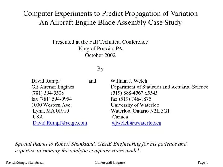
1. Computer Experiments to Predict Propagation of VariationAn Aircraft Engine Blade Assembly Case Study Presented at the Fall Technical Conference King of Prussia, PA October 2002 By Special thanks to Robert Shankland, GEAE Engineering for his patience and expertise in running the analytic computer stress model.

2. Blade Assembly Stress Study • Goals: • A DFSS (design for six sigma) design which meets LCF life requirements • Tolerance requirements for X1, X2, X3 • What was available: • A computer model which evaluates stress for any specific set of X1, X2 and X3 values. Run time ~ 1 hour • Two stress points, Y1 and Y2 as shown. • Two outcomes for each location, mean stress and alternating stress. • Alternating is bigger driver for part low cycle fatigue life. • What was needed: • Non-linear transfer functions for Y1a,b and Y2a,b versus X1, X2 and X3 which could be used for multiple Monte Carlo models, ~1000 iterations each, for stress versus tolerances on X1, X2 and X3. X1=interference fit Y1a,b= notch mean and alternating stress X2=CP rabbet interference fit Y2a,b = rabbet fillet mean and alternating stress X3=CP drop a function of three drops

3. Tolerance meets Customer Need “sigma level” Process Typical Historical Situation 2 xbar +/- 3 s only +/- 2 s fit within tol Robust Design allows Wider Tolerance to meet Customer Need Improved Manufacturing Process “sigma level” Combined Engineering, Manufacturing 6 s Goal 6 xbar +/- 3 s +/- 6 s will fit within tol Six Sigma, Producibility and Robust Design Quality plan relies on inspection. Expect to have rework, scrap and MRB activity. Reaching six sigma goal requires combined Manufacturing/Design Effort Quality plan focus on parameter control and process monitoring. First time yield 100%.

4. Statistical/Design of Experiment Opportunities • Manufacturing Process Improvement: • Screening designs • Factorial designs • Leveraging • EVOP • Quality Improvement metrics • Review by Vice-president • Engineering, meeting Customer Needs and improving producibility: • Quality Function Deployment • Voice of the Customer • Robust Design: • Screening • Factorial • Response Surface Designs • Producibility Scorecards • Review by Vice-president Focus of this presentation

5. Robust Design • Y = Stress or Useful Life • X’s are parameters which impact Y which could include: • Part Key Characteristic values • Environment • Mating part Key Characteristic values • Customer usage pattern • X’s are typically a combination of controllable and noise (uncontrollable) factors • Y = f(XC , XN) • Goals: • Target Y • Minimize sY, that is, variation in Y

6. Non-linear Response 14 12 10 8 Response 6 4 2 0 n 1 2 3 4 5 6 7 X Why Robust Design • Statistical/Engineering method for product/process improvement (Taguchi’s idea) • Two types of factor, control (Xc) and hard to control (Xn or noise) • Control factor levels can change target • Hard to control factors have variation during normal process or usage • Robust design: Set Xc to take advantage of non-linearity in Y = f(Xn) • Design space is typically non-linear

7. Wu and Hamada recommend a two step process • Obtain Transfer Functions: Ybar = f1(XC) sY = f2 (XC) • Typically one finds different sets of X’s in the two transfer functions • If Target is goal: • Minimize variation in Y, the harder objective • Minimize Ybar distance from target • If maximum or minimum is the goal: • Optimize Ybar • Minimize variation in Y • An alternative approach is non-linear optimization of Z where • Z = |Target – Ybar|/ sY Experiments: Planning, Analysis and Parameter Design Optimization, CFJ Wu and M Hamada, Wiley 2000

8. Statistical Issues with Analytic Models • Designing a new part: • Typically done analytically • Often a complex, time consuming process to obtain a result for a single set of parameter values • Examples include finite element analysis models, system models, etc • Leads to serious optimization and simulation issues • Recommended approach: • Run designed experiment, typically Response Surface, to capture non-linear effects • Use RSM transfer function for • Optimization • Simulation to estimate effect of variation in X’s on Y • Statistical Problem: • Analytic models have no random variation, always the same answer for a set of X values • RSM assumes normally distributed error in residuals from model fit • Residuals from analytic model are entirely lack of fit.

9. Case Study was a Learning Process for the GEAE Author • Initial approach: (Note: All results coded for proprietary reasons) • Full Factorial with center-point, 9 computer runs, ~ 9 hours run time • Y’s = life required log transformation • Choose to use Y’s = stress • Interactions and curvature were significant, see Y1a graph below Largest interaction and curvature effects Results led team to an RSM design in 3 factors.

10. RSM Design • Face centered central composite design, illustrated for two factors below • We ran 15 runs, no repeated center-points since computer model has no random variation RSM analysis requires 9+ runs for a 2 factor design, 15+ runs for a 3 factor design. Factor B Factor A

11. RSM Results • Analysis plan and results: • Chose most parsimonious model via backwards selection based on p values • Concerns: • High residuals, especially for Rabbet stress, cause concern. • R-sq not as high as desired • Questions: • Does this transfer function fit well enough for engineering need? • Is there a better way to fit analytic/computer model results

12. Enter Professor William Welch and a Space Filling Design • GEAE author looked for help. Jeff Wu suggested Professor W. Welch of the University of Waterloo • New Experimental Plan: • Space filling design instead of DOE or RSM design • Recommended for computer/analytic experiments • Multiple levels to provide better estimate for non-linear and interaction effects • 33 runs for 3 factors • Doubled the number of runs • Spaces levels for each factor at 1/32nd of the range • Plots below show experimental grid, 2 factors at a time • Computer experiment was run for the 33 sets of conditions (~30 hours of run time)

13. Approximating Random Variable Function Model • Treat Deterministic output Y(x) as a realization of a random function • (stochastic process) • Y(x) = Ybar(x) + Z(x) Sacks et al, Statistical Science, 1989 • Intuition: • Model correlation between Z(x) and Z(x’) for any two input • vectors x and x’ • x close to x’ – correlation large • x far from x’ – correlation small • Leads to a distribution of Y(x) at any x given the Y’s at the • design points • Perform diagnostic tests on model • Accuracy of prediction? Standard error of prediction?

14. Accuracy comparison (e.g., Notch-Alt or Y1b) Error = Y – fitted Y Fitted Y is leave-one-out cross validated (take observation out and predict it) RMSE = 1/n sum (Y – fitted Y)2 -------------------------------------------------- Approximating Cross-Validated Model RMSE --------------------------------------------------- Polynomial – 2nd degree 0.71 Polynomial – 3rd degree 1.04 Random function 0.48 3rd degree polynomial fits even worse than 2nd degree!

15. Actual Diagnostic Checking of Random-Function Model Accuracy assessment: Plot Y versus fitted Y Standard error (se) assessment: Plot (Y – fitted Y) / se(fitted Y) versus fitted Y (Fitted Y is leave-one-out cross validation)

16. Visualization of Input-Output Relationships e.g. Y1b as a function of RetArm Other two inputs (CPRabbet and CPDrop) averaged out

17. Propagating Variation Through the Random Function Model CPRabbet, CPDrop, RetArm have independent N(mu, sigma) distributions e.g., set mu = center of range Sample CPRabbet, CPDrop, RetArm and pass through model to get a distribution of e.g., Y1b values

18. Conclusions • RSM approach: • Good starting point • Will work fine for Ybar and simple underlying Physics • Space Filling Design: • Allows us to model responses with very nonlinear underlying • Physics • Random-function model: • Provides valid standard errors of prediction • Can adapt to nonlinearities in data • Fast, so can quickly propagate variation • inputs => outputs • via Monte Carlo