Download

1 / 17
170 likes | 187 Views
Explore an innovative strategy leveraging node density to extend network lifespan, with an emphasis on coverage efficacy, fault tolerance, and energy efficiency. Examine the protocol's working schedule determination and execution in detail.

E N D
Differentiated Surveillance for Sensor Networks Ting Yan, Tian He, John A. Stankovic CS294-1 Jonathan Hui November 20, 2003
Idea • Exploit node density/redundancy to maximize effective network lifetime. • Degree of coverage matters! • Sensing constraints • Fault tolerance
Assumptions • Static placement • Localization • Time Synchronization • Uniform expected node lifetime • For simplicity of describing protocol? • Nodes on 2D plane • Circular sensing radius r • Communication range > 2r
Basic Protocol • Initialization Phase • Localization, Time Sync, Determine Working Schedule (T, Ref, Tfront, Tend) • Sensing Phase • Nodes power on and off based on working schedule Round 0 (T) Round 1 (T) Round i (T) Ref Ref Ref t Tfront Tend Tfront Tend Tfront Tend Sensing Phase Init Phase
Basic ProtocolDetermining Working Schedule • Goal: Each node determines its own working schedule such that all points within sensor coverage are covered for all time. • Approach: Represent sensor coverage with grid of points
Basic ProtocolDetermining Working Schedule • Reference Point Scheduling Algorithm • Randomly choose Ref from [0, T) and broadcast to all nodes within 2r. • For each discrete point • Order neighboring Ref times and calculate • Tfront = [Ref(i)-Ref(i-1)]/2 • Tend= [Ref(i+1)-Ref(i)]/2 • Final schedule = union of schedules for all points RefC RefA RefB Point 1 RefC RefA RefB Node A: RefD RefA RefE RefD RefE Point 2
Example (a = 2) Example (a = 3) RefB RefC RefB RefC RefA RefA A A B B Uh-Oh! C C Enhanced Protocolwith Differentiation Example (a = 1) • Working schedule for a desired coverage of degree a. • (T, Ref, Tfront, Tend, a) • Working period defined as: • Power On: • Power Off: RefB RefC RefA A B C
Design Issues • Possible blind spots with discrete points • Choose points within sensing range conservatively • Offset in time synchronization • Power on (off) slightly earlier (later) • Irregular sensing regions • Okay, as long as sensing regions of neighboring nodes are known • But also requires knowledge of orientation • Fault Tolerance • Awake nodes use heartbeat messages to detect failed nodes • If a node fails, wakeup all nodes within 2r and reschedule. • What if communication range < 2r?
Extensions and Optimizations • Second Pass Optimization • After determining working schedule, broadcast schedule to all nodes within 2r. • The node which has the longest schedule: • Minimize Tfront and Tend while maintaining sensing guarantee • Rebroadcasts new schedule • Done when every node has recalculated schedule or when no more can be done.
Extensions and Optimizations • Multi-Round Extension for Energy Balance • Calculate M schedules each with different Ref values during Init Phase. • Rotate schedules during Sensing Phase. RefB RefC RefA RefB RefC RefA RefA RefB RefC RefA RefC RefB A B C Schedule 1 Schedule 2 Schedule 3 Schedule 4
Evaluation • Simulation parameters • Nodes distributed randomly with uniform distribution in 160mX160m field. • Results taken from center 140mX140m to avoid edge effects • Sensing range = 10m • Communication range = 25m • Ideal conditions • Fault tolerance included? • Compare against sponsored approach
Evaluation • Total energy consumption nearly constant with changes in density. • Variation in total energy consumed decreases with greater densities. • What’s happening with the sponsored approach?
Evaluation • Half-life increases linearly as density increases. • Coverage provided for longer period of time.
Evaluation • Energy consumption increases linearly with different degrees. • Energy consumption constant with different densities. • Degree of coverage provided >= a. • a only guarantees a lower bound.
Comments • Localized algorithm? • But still requires time synchronization and doesn’t support mobility • Inflexible • mobility not supported, schedules are fixed • No notion of the “goodness” of a node • Nodes that have more energy should take up a larger portion of the working schedule • Difficult to reliably broadcast Ref values to all 2r neighbors in a dense network • Only have one chance to get it right! • Worse in cases where communication range < 2r (i.e. acoustic sensors)
Comments • Working schedules determined without taking other schedules and protocols into account • How does it affect other protocols (i.e. TDMA)? • Comparison to Sponsored Coverage unfair • Sponsored Coverage supports fault tolerance, limited mobility, and is more adaptable • Ability to specify degree of coverage • But current algorithm doesn’t correctly guarantee with a > 2! • Fault tolerance relies on communication range > 2r for heartbeat messages
Conclusion • Pros • Improved performance in lifetime and workload balance • Specify a degree of coverage • Cons • No upper bound on degree estimation • Inflexible • Static working schedule, static nodes, time synchronization, reliable communication