Download
1 / 20
210 likes | 393 Views
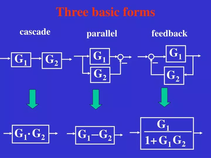
Three basic forms. G 1. G 1. G 1. G 2. G 2. G 2. G 1. G 1. G 2. G 1. G 2. G 2. G 1. 1+. cascade. parallel. feedback. behind a block. y. x 1. y. x 1. G. G. ±. ±. x 2. x 2. G. Ahead a block. y. y. x 1. x 1. G. G. ±. ±. x 2. x 2. 1/G.

E N D
Three basic forms G1 G1 G1 G2 G2 G2 G1 G1 G2 G1 G2 G2 G1 1+ cascade parallel feedback
behind a block y x1 y x1 G G ± ± x2 x2 G Ahead a block y y x1 x1 G G ± ± x2 x2 1/G 2.6 block diagram models (dynamic) 1. Moving a summing point to be: 2.6.2.2 block diagram transformations
behind a block x1 x1 y y G G x2 x2 1/G ahead a block x1 x1 y y G G x2 x2 G 2.6 block diagram models (dynamic) 2. Moving a pickoff point to be:
Summing points x3 x3 + x1 y + x1 y - - x2 x2 Pickoff points y y x1 x2 x2 x1 2.6 block diagram models (dynamic) 3. Interchanging the neighboring—
1. Neighboring summing point and pickoff point can not be interchanged! 2. The summing point or pickoff pointshould be moved to the same kind! 3. Reduce the blocksaccordingto three basic forms! 2.6 block diagram models (dynamic) Notes: 4. Combining the blocks according to three basic forms. Examples:
Moving pickoff point H2 G3 G4 G2 G1 1 H2 G4 H3 G3 G4 G1 G2 H1 H3 H1 Example 2.17 a b
Moving summing point G3 G3 G1 G1 G2 G2 H1 H1 G1 Move to the same kind Example 2.18
Disassembling the actions G4 G1 G2 G3 H3 H1 G4 G1 G2 G3 H3 H1 H3 H1 Example 2.19
G Chapter 2 mathematical models of systems Block diagram reduction ——is not convenient to a complicated system. 2.7 Signal-Flow Graph Models Signal-Flow graph —is a very available approachto determine the relationship between the input and output variables of a sys-tem,only needing a Mason’s formulawithout the complex reduc-tion procedures. 2.7.1 Signal-Flow Graph only utilize two graphical symbols for describing the relation-ship between system variables。 Nodes, representing the signals or variables. Branches, representing the relationship and gain Between two variables.
f c x0 x4 x1 x3 x2 g a d h b e 2.7 Signal-Flow Graph Models Example 2.20: 2.7.2 some terms of Signal-Flow Graph Path — a branch or a continuous sequence of branches traversing from one node to another node. Path gain — the product of all branch gains along the path.
Loop gain —— the product of all branch gains along the loop. Touching loops ——more than one loops sharing one or more common nodes. Non-touching loops — more than one loops they do not have a common node. 2.7 Signal-Flow Graph Models Loop —— a closed path that originates and terminates on the same node, and along the path no node is met twice. 2.7.3 Mason’s gain formula
f c x0 x4 x1 x3 x2 g a d h b e 2.7 Signal-Flow Graph Models Example 2.21
and G(s) 2.7 Signal-Flow Graph Models 2.7.4 Portray Signal-Flow Graph based on Block Diagram Graphical symbol comparison between the signal-flow graph and block diagram: Block diagram Signal-flow graph G(s)
H1 C(s) R(s) X1 - E(s) X3 G1 G3 G4 G2 - X2 - H2 H3 -H1 R(s) 1 G2 X2 X3 C(s) G3 X1 G4 E(s) G1 -H2 -H3 2.7 Signal-Flow Graph Models Example 2.22
-H1 X2 R(s) X1 X3 1 C(s) E(s) G1 G2 G4 1 G3 -H2 -H3 2.7 Signal-Flow Graph Models
- X1 Y1 - G1 + + C(s) R(s) E(s) + - - X2 G2 Y2 - -1 1 -1 X1 Y1 G1 -1 1 -1 C(s) E(s) R(s) 1 1 1 Y2 X2 G2 -1 2.7 Signal-Flow Graph Models Example 2.23
-1 X1 Y1 G1 -1 1 -1 C(s) E(s) R(s) 1 1 1 1 Y2 X2 G2 -1 -1 2.7 Signal-Flow Graph Models 7 loops: 3 ‘2 non-touching loops’ :
-1 X1 Y1 G1 -1 1 -1 C(s) E(s) R(s) 1 1 1 1 Y2 X2 G2 -1 -1 2.7 Signal-Flow Graph Models Then: 4 forward paths:
2.7 Signal-Flow Graph Models We have