Download
1 / 15
150 likes | 269 Views
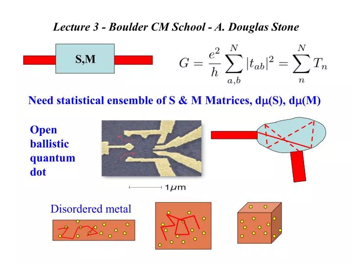
S,M. Disordered metal. Lecture 3 - Boulder CM School - A. Douglas Stone. Need statistical ensemble of S & M Matrices, d (S), d (M). Open ballistic quantum dot. Dyson. Simplest possibility: completely uniform on the matrix space.

E N D
S,M Disordered metal Lecture 3 - Boulder CM School - A. Douglas Stone Need statistical ensemble of S & M Matrices, d(S), d(M) Open ballistic quantum dot
Dyson Simplest possibility: completely uniform on the matrix space • This is possible for unitary S-matrix (circular ensembles), • Not for pseudo-unitary M-matrix (non-compact space) Hypothesis: P(S) = d(S)/V for chaotic quantum dot dS2 = Tr{dSdS†} = ∑ij gij dqiqj => d(S) = (det[g])1/2∏idqi We need a parameterization in term of {Tn}
MesoNoise WL UCF Coulomb Gas analogy Circular ensemble: take V = 0, P({Tn}) only from invariant measure;what to do with jpd? For Var(g) need Need 1-pt and 2-pt correlation fcns of the jpd of {Tn}
Use recursion relations, asymptotic form of pn : (normalized to N - so that G = (e2/h) T Many methods to find these fcns and the two-pt corr. fcn is “universal” upon rescaling if only logarithmic correlations Nice approach for =2 is method of orthogonal polynomials pn= orthog poly, choose Legendre, [0,1] Same method gives K(T,T’) in terms of pN pN-1
(T)/N 0 1 T What do we expect for this system? Classical symmetry betweeen reflection and transmission => <R> = <T> = N/2 Need to go to next order in N-1 to get WL effect
Tr{r r†} = R SCOE =UUT U Coherent backscattering Off-diagonal correlations Coherent backscattering < R >COE GWL = -(2e2/h)(1/4) The Mystery Can get order 1/N effects easily for the circular ensemble - do averages over unitary group U(2N) Similarly Var(g) = (1/8)
CB only Actual data from ballistic junction -M. Keller and D. Prober 1995 Agrees well with experiment and simulations
RMT =2 Variance of g for a quantum dot (Chan et al., 95),Note factor of two reduction when B ≠ 0 (=2)
M2 M1 M = M1M2 dM(dL) M(L) DMPK Equation Disordered Wires No T R symmetry <g> = N(l/L), l = mfp<R> ≈ N, l << L L Use M, not S Parameterize M(L) with polar decomposition PL+dL= PL(M) PdL(dM)(ML+dL - ML• dMdL) “isotropic”
{n} = Inverse localization lengths 1D case solved early(1959), Mello (88,91), Beenakker (93),RMP (97) Qualitative picture: Imry (86), open and closed channels
1/2L UCF: Var(g) = 2/(15) , gWL = -1/3 1 2 N Nopen Nclosed g ≈ Nopen = Nl/L => 1 = 1/(2Nl) • When L > 2Nl => g = exp[-L/(Nl)] => quasi-1d localization, = Nl. • Fixed N (width) and increasing L always leads to localization. Var(g) = Var(Nopen) ≈ 1 (spectral rigidity, P({n}) ∏open | n - m| )
closed Tunnel barrier closed open Chaotic junction closed disordered open Disordered wire Ballistic/chaotic Eigenvalue density
s y y’ x x’ b a sinb = ±bπ/kW Semiclassical Method for Ballistic Junctions Obtained by stationary phase integration of FT of Gscl(r,r’,t);0∫ T Ldt Ss (E) = r∫ r’pdq = (h/2π)kLs (for billiard) Now do ∫∫ dydy’ for tab by stationary phase:
g = N/2 comes from terms s=u, WL correction from s≠ u, but not simply from time-reversed pairs of path Conductance fluctuations come from random interference of paths, sensitive to B, k - Var(g) ≈ 1 comes from interference of all paths, require correlated actions for different paths Fundamentally different from familiar speckle patterns
Look at diagonal terms, s=u; Can get dynamical scales just from diagonal terms Sum starts to decay when kLs ≈ π => kc = < π/L> = cFor diffusive case Ls = vf tD => kc = Eth/hvf Similar analysis give Bc = (h/e)/<Aencl> Quantitative approach next time.