CAD Mesh Model Segmentation by Clustering

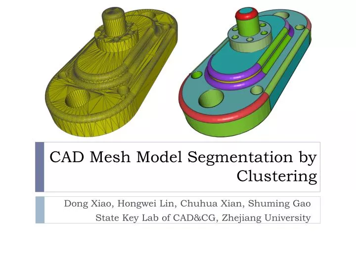
1. CAD Mesh Model Segmentation by Clustering Dong Xiao, Hongwei Lin, Chuhua Xian, ShumingGao State Key Lab of CAD&CG, Zhejiang University

2. Introduction

3. Mesh Segmentation

4. CAD Mesh Model

5. Related Work • V. Sunil, S. Pande, Automatic recognition of features from freeform surface CAD models, Computer-Aided Design 40 (2008) 502–517. • Divide the model into dense and coarse parts via feature edge detection. • Dense regions are segmented based on the signs of gauss curvature and mean curvature. • Coarse regions are segmented into planar, cylindrical and ruled regions via a heuristic method.

6. Our Work • The CAD mesh model is classified into sparse and dense regions by the agglomerative hierarchical clustering method. • The sparse region is partitioned into planar, cylindrical, and conical regions by the Gauss map and randomized Hough transformation. • The dense region is segmented by performing the mean shift operation on the mean curvature field.

7. Dense and Sparse Region Clustering

8. Triangles in Dense and Sparse Regions

9. Clustering Triangles • Calculate m = Area × EdgeRatio for each triangle, and store them in a sorted list. Treat each one as a cluster initially. • Among all pairs of adjacent clusters, pick out the pair with the minimum distance and merge them to one cluster. The distance is: d = | log m1 - log m2 | • Continue step 2 until there are only two clusters left.

10. Clustering Triangles

11. Issue of Automatic Clustering

12. Segmentation of the Sparse Region

13. Planar Patch Recognition • Merge the adjacent sparse triangles with the same normal. (Inner product >= 1 – 10-5) • Some small triangles that are recognized as dense triangles by mistake are also merged if they are in the same plane with a neighboring sparse triangle.

14. Gauss Map • The planar region is mapped to a point on the Gauss sphere surface. The cylindrical and conical regions are mapped to great and small circles on the Gauss sphere surface, respectively.

15. Gauss Map • Map the normalized normals of these merged planar patches and non-merged triangular patches into the Gauss sphere, then use randomized Hough transformation to recognize the planes.

16. Randomized Hough Transformation • Randomly choose 3 points from the data points on the Gauss sphere, insert the plane constructed from them into the accumulator. • Repeat step 1 until a plane appears a number of times in the accumulator (e.g. 1,000 times). Report the plane and remove all points on the plane from the data set. • Repeat step 1 until there’re no enough points left (6). • In the accumulator, similar planes are merged.

17. Postprocessing • A great circle in the Gauss sphere may contain planar patches that: • are not connected in the model; • form several connected cylindrical regions with different but parallel axes; • form a cylindrical region and a tangential planar region; • is inside another cylindrical region with different direction. • Employ constraints on connectivity, dihedral angel (20˚) and area ratio (5 or 2.5) to recognize the real cylindrical regions. • The same for conical regions.

18. Current Results

19. Segmentation of the Dense Region

20. Mean Shift Normal & Curvature

21. Curvature Computation in Triangles

22. Mean Shift • Mean-shift is a non-parametric feature-space analysis technique. • It is a procedure for locating the maxima of a density function given discrete data sampled from that function. It is useful for detecting the modes of this density.

23. Mean Shift on Curvature • Mean curvature ci at the center Pi of each triangle constitute the mean curvature fieldχ = {xi = (Pi, ci), i = 1, 2, …, n} in R4.

24. Mean Shift on Curvature • Mean shift clustering: • Initialize yi[0]with xi, i = 1, 2, …, n; • Compute y[j + 1] = y[j] + m(y[j]) until convergence. • Connected triangles with the same convergence point are segmented as one region. • Use a k-D tree to speed up the process.

25. Implementation and Results

26. Results

27. Results

28. Results

29. Comparison

30. Statistics of Segmentation

31. Parameters and Time for Dense Regions

32. Conclusions and Future Work

33. Pros • Clustering the triangles into sparse and dense parts is simpler and more robust than the feature edge detection method. • Recognizing the cylindrical and conical regions via Gauss map and Hough transformation is more robust than the heuristic method. • Segmentation of the dense regions by mean shift curvature can separate different blending surfaces well.

34. Cons and Future Work • Influence of neighboring sparse regions and the shapes of triangles in mean curvature computation. • Improve the computation method. • The parameters of mean shift is not easy to choose. • Automatically control them. • Can not distinguish a convex cylindrical region with an adjacent concave cylindrical region if both of them have a bit noise. • Need a robust method to distinguish them.

35. Q&A

36. Thank You!