Download

1 / 12
120 likes | 138 Views
Explore the Equilibrium Business Cycle Model by examining fluctuations in output and testing its fit with real-world data. Discover how technology shocks impact wages, rents, consumption, and investment, and analyze predictions against actual outcomes. This lecture delves into the implications of permanent changes in technology and the observed patterns in key variables. The session highlights the cyclical nature of wages, rental costs, consumption, and investment, shedding light on understanding economic fluctuations. Join us as we bridge theoretical models with empirical evidence to enhance our understanding of macroeconomic dynamics.

E N D
Lecture 12: The Equilibrium Business Cycle Model L11200 Introduction to Macroeconomics 2009/10 Reading: Barro Ch.8 18 February 2010
Introduction • Last time: • Completed the macroeconomic model by analysing how consumption impacted investment • Today • Begin to apply the model by studying the fluctuations in output more closely • Test whether the model fits the data
‘Equilibrium Business Cycle’ • The model we have constructed is known as an ‘Equilibrium Business Cycle Model’ • ‘Equilibrium’ because markets are continually in equilibrium • ‘Business Cycle’ because it seeks to explain the cycle of fluctuations known by this name • Aims to explain economic fluctuations
Fluctuations • There are clearly fluctuations, but how do we measure them? • GDP is trended upwards, but deviates around that trend • Can estimate trend and deviation using filtering techniques • Classify ‘recessions’ as periods of growth which are significantly lower than trend growth
Testing the Model • Fluctuations in technology: • Part one of the course established that growth in A is the best explanator of long-run economic growth • Idea here: fluctuations in A are best explanator of fluctuations in growth • So positive and negative shocks to technology drive short-term expansions and contractions
Testing the Model • Test this idea with the following questions • If fluctuations in output are caused by fluctuations in technology, what does that imply for fluctuations in wages, rents, consumption, investment, unemployment, capital utilisation? • Does the data conform with the predictions of the model?
Technology Shocks • Our production function is subject to shocks in A • Positive shock to A means that for a given K,L output increases (so MPL and MPK increase) • Negative shock to A means that for a given K,L output decreases (so MPL and MPK decrease)
Implications: • Increase in technology level • Raises demand for labour, with inelastic supply this causes increase in real wage w/P • Raises demand for capital, with inelastic supply this causes increase in rental cost R/P • Increase in rental cost means i also increases
Implications for Consumption • Interest rate i increases • Intertemporal substitution effect encourages households to save, consumption should fall • But if A is permanent, large positive income effect encourages consumption to increase • So net effect is increase in consumption when technology shock hits
Predictions • So, if technology is driving output fluctuations • Wages should rise when output rises and fall when output falls • Interest rates should rise when output rises and fall when output falls • Consumption and Investment should both rise when output rises and fall when output falls • That is, all of these variables should be procyclical (instead of counter-cyclical)
Outcome • Is the data consistent with a model in which permanent changes to A drive output • Wages a procyclical (as predicted) • Rental cost is procyclical (as predicted) • Consumption is procyclical (as predicted) and less variable than GDP • Investment is procyclical (as predicted) and more variable than GDP • How to explain the last two patterns?
Summary • Began testing model of fluctuations on data • Permanent changes in A imply a particular pattern for key variables • This pattern appears evident in the data: supports the model • Next time: no longer assume L and K are fixed • Wages are procyclical – but so is employment (i.e. L is not fixed!) how do we explain this?