Download
1 / 55
560 likes | 868 Views
Practical logarithmic rasterization for low error shadow maps. Brandon Lloyd UNC-CH Naga Govindaraju Microsoft Steve Molnar NVIDIA Dinesh Manocha UNC-CH. Shadows are important aid spatial reasoning enhance realism can be used for dramatic effect

E N D
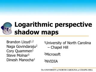
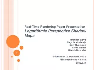
Practical logarithmic rasterization for low error shadow maps Brandon Lloyd UNC-CH Naga Govindaraju Microsoft Steve Molnar NVIDIA Dinesh Manocha UNC-CH
Shadows are important aid spatial reasoning enhance realism can be used for dramatic effect High quality shadows for real-time applicationsremains a challenge Shadows
Shadow approaches • Raytracing [Whitted 1980] • not yet real-time for complex, dynamic scenes at high resolutions • Shadow volumes [Crow 1977] • can exhibit poor performance on complex scenes
Light Shadow maps [Williams 1978] Eye
Logarithmic perspective shadow maps (LogPSMs) [Lloyd et al. 2007] Standard shadow map LogPSM
Logarithmic perspective shadow maps (LogPSMs) [Lloyd et al. 2007] Standard shadow map LogPSM
Goal linear rasterization logarithmic rasterization Perform logarithmic rasterization at rates comparableto linear rasterization
Outline • Background • Handling aliasing error • LogPSMs • Hardware enhancements • Conclusion and Future work
Requires more bandwidth Decreases shadow map rendering performance Requires more storage Increased contention for limited GPU memory Decreased cache coherence Decreases image rendering performance High resolution shadow maps Poor shadowmap querylocality
Sample at shadow map query positions No aliasing Uses irregular data structures requires fundamental changes to graphics hardware [Johnson et al. 2005] Irregular z-buffer [Aila and Laine 2004;Johnson et al. 2004]
Adaptive partitioning • Adaptive shadow maps [Fernando et al. 2001] • Queried virtual shadow maps[Geigl and Wimmer 2007] • Fitted virtual shadow maps [Geigl and Wimmer 2007] • Resolution matched shadow maps [Lefohn et al. 2007] • Multiple shadow frusta [Forsyth 2006]
Adaptive partitioning • Requires scene analysis • Uses many rendering passes
Match spacing between eye samples Faster than adaptive partitioning no scene analysis few render passes Scene-independent schemes eye sample spacing
Cascade shadow maps • Cascaded shadow maps [Engel 2007] • Parallel split shadow maps [Zhang et al. 2006]
Perspective shadow maps (PSMs) [Stamminger and Drettakis 2002] Light-space perspective shadow maps (LiSPSMs) [Wimmer et al. 2004] Trapezoidal shadow maps (TSMs)[Martin and Tan 2004] Lixel for every pixel [Chong and Gortler 2004] Projective warping
Not necessarily the best spacing distribution Projective warping PSM LiSPSM moderate error high error y x moderate error low error
Logarithmic+perspective parameterization Logarithmictransform Perspectiveprojection Resolutionredistribution
Bandwidth/storage savings - near and far plane distances of view frustum *shadow map texels / image pixels
LogPSMs have lower maximum error more uniform error Image resolution: 5122 Shadow map resolution: 10242 f/n = 300 Grid lines for every 10 shadow map texels Color coding for maximum texel extent in image Single shadow map LogPSM LogPSM LiSPSM LiSPSM LogPSM
More details Logarithmic perspectiveshadow maps UNC TR07-005 http://gamma.cs.unc.edu/logpsm
Outline • Background • Hardware enhancements • rasterization to nonuniform grid • generalized polygon offset • depth compression • Conclusion and Future work
setup Graphics pipeline vertex processor memory interface clipping rasterizer fragment processor alpha, stencil, & depth tests depth compression color compression blending
Rasterization • Coverage determination • coarse stage – compute covered tiles • fine stage – compute covered pixels • Attribute interpolation • interpolate from vertices • depth, color, texture coordinates, etc.
Signs used to compute coverage Water-tight rasterization Use fixed-point fixed-point “snaps” sample locations to an underlying uniform grid Edge equations +-+ -++ +++ ++-
Attribute interpolation • Same form as edge equations:
y' y x x Logarithmic rasterization light space linear shadow mapspace warped shadow mapspace Linear rasterization with nonuniform grid locations.
Edge and interpolation equations • Monotonic • existing tile traversal algorithms still work • optimizations like z-min/z-max culling still work
Full parallel implementation Coverage determinationfor a tile Full evaluation
Incremental in x Coverage determination for a tile 1 2 Full evaluation Incremental x Per-triangle constants
Generalized polygon offset light - depth slope - smallest representable depth difference constant texelwidth
Generalized polygon offset light - depth slope - smallest representable depth difference constant texelwidth not constant
Generalized polygon offset • Do max per pixel • Split polygon • Interpolate max at end points
store compressed yes tile table fits in bit budget? no store uncompressed Depth compression • Important for reducing memory bandwidth requirements • Exploits planarity of depth values • Depth compression survey [Hasselgren and Möller 2006] depth compressor tile
Depth compression - Standard compressed untouched clamped Resolution: 512x512 Linear depth compression Our depth compression
Depth compression - LiSPSM compressed untouched clamped Resolution: 512x512 Linear depth compression Our depth compression
Depth compression - LogPSM compressed untouched clamped Resolution: 512x512 Linear depth compression Our depth compression
Depth compression – LogPSM Higher resolution compressed low curvature untouched clamped Resolution: 1024x1024 Linear depth compression Our depth compression
Δx Δx Δx z0 Δy Δy Δx Δx Δx Δx d d Δy Δx Δx Δx Δy d d Δy Δx Δx Δx Δy Δy Our compression scheme z0 d d d d a1 a0 Differentialencoding Anchor encoding 128-bit allocation table
Test scenes • Town model • 58K triangles • Robots model • 95K triangles • Power plant • 13M triangles • 2M rendered
Compression methods tested • Anchor encoding[Van Dyke and Margeson 2005] • Differential differential pulse code modulation (DDPCM)[DeRoo et al. 2002] • Plane and offset[Ornstein et al. 2005] • Hasselgren and Möller [2006]
Compression results • Average compression over paths through all models • Varying light and view direction
Anchor encoding best linear method higher tolerance for curvature Compression results
Summary of hardware enhancements • Apply F(y) to vertices in setup • log and multiply-add operations • Evaluators for G(y’) • exponential and multiply-add operations • Possible increase in bit width for rasterizer • Generalized polygon offset • New depth compression unit • can be used for both linear and logarithmic rasterization
Feasibility • Leverages existing designs • Trades computation for bandwidth • Aligns well with current hardware trends • computation cheap • bandwidth expensive
Conclusion • Shadow maps • Handling errors requires high resolution • Logarithmic rasterization • significant savings in bandwidth and storage • Incremental hardware enhancements • Rasterization to nonuniform grid • Generalized polygon offset • Depth compression • Feasible • leverages existing designs • aligns well with hardware trends
Future work • Prototype and more detailed analysis • Greater generalization for the rasterizer • reflections, refraction, caustics,multi-perspective rendering [Hou et al. 2006; Liu et al. 2007] • paraboloid shadow maps for omnidirectional light sources [Brabec et al. 2002] • programmable rasterizer?
Acknowledgements • Jon Hasselgren and Thomas Akenine-Möller for depth compression code • Corey Quammen for help with video • Ben Cloward for robots model • Aaron Lefohn and Taylor Holiday for town model
Acknowledgements • Funding agencies • NVIDIA University Fellowship • NSF Graduate Fellowship • ARO Contracts DAAD19-02-1-0390 and W911NF-04-1-0088 • NSF awards 0400134, 0429583 and 0404088 • DARPA/RDECOM Contract N61339-04-C-0043 • Disruptive Technology Office.