Download
1 / 21
210 likes | 338 Views
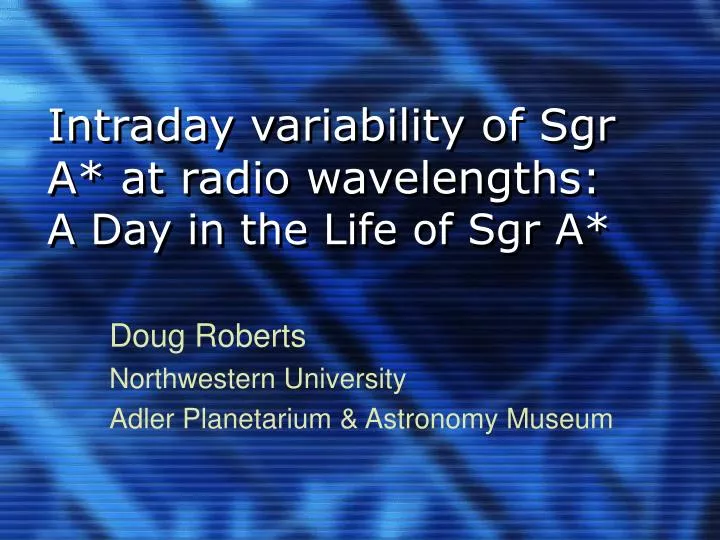
Intraday variability of Sgr A* at radio wavelengths: A Day in the Life of Sgr A*. Doug Roberts Northwestern University Adler Planetarium & Astronomy Museum. Collaborators. Farhad Yusef-Zadeh – Northwestern University Geoff Bowers – University of California Berkeley

E N D
Intraday variability of Sgr A* at radio wavelengths:A Day in the Life of Sgr A* Doug Roberts Northwestern University Adler Planetarium & Astronomy Museum
Collaborators • Farhad Yusef-Zadeh – Northwestern University • Geoff Bowers – University of California Berkeley • Craig Heinke – Northwestern University
Motivation: Campaign • Started as part of multi-wavelength campaign in March 2004. • Follow-up observations of Sgr A* and nearby X-ray/radio transient were done throughout 2004-05.
Motivation: Previous determinations of radio variability • Long term radio variability • 106 day variability 15 & 22 GHz (Zhao et al. 2001) • 2.5 yr observations at 15, 22 & 43 GHz suggest bimodal flux densities and spectral indices (Herrnstein et al. 2004) • Hourly variability at high frequencies: • 1.5 hour (x 2 flux) flare at 100 & 140 GHz (Miyazaki et al. 2004) • 2.5 hour variability at 100 GHz (Mauerhan et al. 2005)
Radio observations used various telescopes (5-83 GHz) BIMA (83 GHz) ATCA (17, 19 GHz) VLA (5, 22, 43 GHz)
Observations designed to observe intraday variability • All observations were done with frequent pointings between Sgr A* and a nearby (3º) calibrator (cycled between 90 seconds on source and 30 seconds on calibrator). • Less frequent observations of a strong calibrator further away (10º). • Pointing scans every hour. • Tipping scan to determine the atmospheric opacity at the beginning of the run.
Lots of data! • 32 Datasets • Each about 5 hr in length • 20 GB of raw data
Data analysis • Phase calibration on calibrators applied before ordinary calibration. • Phase self-cal on Sgr A*. • Flux of Sgr A* determined by fitting point source model in visibility plane, using only long spacing that filter out diffuse emission from Sgr A West.
First look • Radio variability of 5-10% at various timescales. • High time resolution samples show few percent variation every sample (2 minutes). • Significant day-to-day variability. Example light curve – 1 day Example light curve – 1 week
Calibration issues • Is variation real or artifact of observation or problems with calibration?
Calibration issues • Is variation real or artifact of observation or problems with calibration? • Variation within an observation is pretty reliable. • Day-to-day variation is harder to verify.
Analysis of light curve • Lomb-Scargle analysis of each light curve separately. • Monte Carlo simulation of red noise – P(f) ~ f-1 – using the statistics of the relevant observation – following technique of Mauerhan et al.
Interpretation of variability distribution • Lower limit to time scale for variability of 2.5 hr. • Similar to peak in OVRO 83 GHz power spectrum. • If the time scale for this variability is related to dynamics of emitting gas, this suggests a dynamical radius of 10 Rs.
Radio flare simultaneously detected at 22 & 43 GHz • 43 GHz emission leads 22 GHz by about 20 minutes. • Spectral index is steeper at higher frequencies and during flares, consistent with Herrnstein et al. (2004). • Consistent with expansion of self-absorbed synchrotron source.
Scintillation vs. intrinsic changes • Similar shape of light curve and delay between 22 & 43 GHz. • Scintillation effects cannot explain this delay.
Summary • Typical variability within one day is 5-10%. • Variability on various timescales from 2 hr to 5 hr (to 10 hr for long ATCA tracks). • Lower limit to dynamic length scale is around 10 Rs. • Delay in 22 GHz and 43 GHz observations of flare. • Model of variability suggests high optical depth from expanding synchrotron source.