Download
1 / 12
120 likes | 141 Views
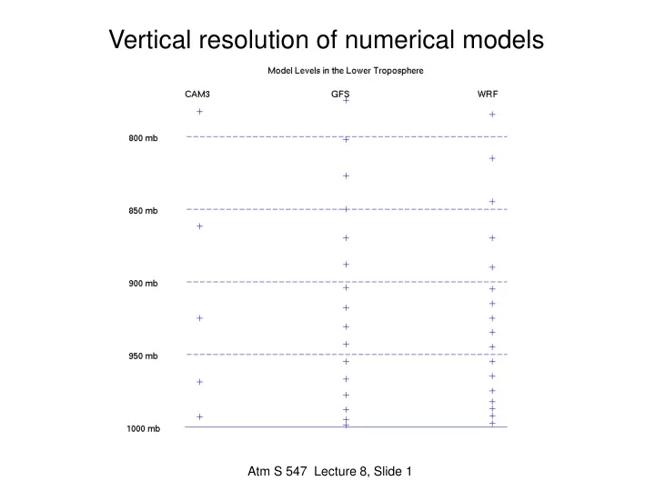
Vertical resolution of numerical models. Observational support for CBL entrainment closure. Mixed-layer model of dry convective BL. Real (Wangara). MLM idealization. t 2. + (z). h 2. t 1. 1. z. h 1. H s. 2. 1. Galperin (1988) stability functions.

E N D
Vertical resolution of numerical models Atm S 547 Lecture 8, Slide 1
Observational support for CBL entrainment closure Atm S 547 Lecture 8, Slide 2
Mixed-layer model of dry convective BL Real (Wangara) MLM idealization t2 +(z) h2 t1 1 z h1 Hs 2 1 Atm S 547 Lecture 8, Slide 3
Galperin (1988) stability functions Atm S 547 Lecture 8, Slide 4
Profile vs. forcing-driven turbulence parameterization Mellor-Yamada turbulence closure schemes are profile-driven: Nonturbulent processes destabilize u,v, profiles. The unstable profiles develop turbulence. • Such schemes (except 1st order closure) can be numerically delicate: Small profile changes (e.g. from slightly stable to unstable strat) can greatly change KH,M(z), turbulent fluxes, hence turbulent tendencies. This can lead to numerical instability if the model timestep t is large. • TKE schemes are popular in regional models (t ~ 1-5 min). • Most models use first-order closure for free-trop turbulent layers. Alternate K-profile approach (next) is forcing-driven: KH,M(z) are directly based on surface fluxes or heating rates. • More numerically stable for long t • Hence K-profile schemes popular in global models (t ~ 20-60 min). • However, K-profile schemes only consider some forcings (e. g. surface fluxes) and not others (differential advection, internal radiative or latent heating), so can be physically incomplete. Atm S 547 Lecture 8, Slide 5
K-profile method • Parameterize turbulent mixing in terms of surface fluxes (and possibly other forcings) using a specified profile scaled to a diagnosed boundary layer height h. • Example: Brost and Wyngaard (1978) - for stable BLs (Z = z/h) • h empirically diagnosed using threshold bulk Ri, e. g. Vogelezang&Holtslag 1996 where ‘sfc’ = 20 m Atm S 547 Lecture 8, Slide 6
A challenge to downgradient diffusion: Countergradient heat transport • In dry convective boundary layer, deep eddies transport heat • This breaks correlation between local gradient and heat flux • LES shows slight q min at z=0.4h, but w’q’>0 at z<0.8h • ‘Countergradient’ heat flux for 0.4 < z/h < 0.8…first recognized in 1960s by Telford, Deardorff, etc. Cuijpers and Holtslag 1998 Atm S 547 Lecture 8, Slide 7
Nonlocal schemes This has spawned a class of nonlocal schemes for convective BLs (Holtslag-Boville in CAM3, MRF/Yonsei in WRF) which parameterize: Atm S 547 Lecture 8, Slide 8
Derivation of nonlocal schemes Heat flux budget: B S T M P Neglect storage S Empirically: For convection, a=0.5, so Take = 0.5h/w* to get zero gradient at 0.4h. Holtslag and Moeng (1991) Atm S 547 Lecture 8, Slide 9
Nonlocal parameterization, continued where This has the form Although the derivation suggests is a strong function of z, the parameterization treats it as a constant evaluated at z = 0.4h to obtain the correct heat flux there with d/dz = 0: The eddy diffusivity can be parameterized from vert. vel. var.: With cleverly chosen velocity scales, this can be seamlessly combined with a K-profile for stable BLs to give a generally applicable parameterization (Holtslag and Boville 1993). Atm S 547 Lecture 8, Slide 10
Comparison of TKE and nonlocal K-profile scheme UW TKE scheme (Bretherton&Park 2009) vs. Holtslag-Boville. • GABLS1 (Beare et al. 2004) • Linear initial profile • ug = 10 m/s • sfc cooled at 0.25K/hr • 8-9 hr avg profiles • UW and HB both do well • Default CAM3 has too much free-trop diffusion, causing BL overdeepening Bretherton and Park 2009 Atm S 547 Lecture 8, Slide 11
CBL comparison • Sfc heating of 300 W m-2 • No moisture or mean wind • UW TKE scheme with entrainment closure and HB scheme give similar results at both high and low res. • Overall, can get comparably good results from TKE and profile-based schemes on these archetypical cases. Bretherton and Park 2009 Atm S 547 Lecture 8, Slide 12