Download
1 / 46
1.25k likes | 3.1k Views
Image Interpolation. Introduction What is image interpolation? Why do we need it? Interpolation Techniques 1D zero-order, first-order, third-order 2D zero-order, first-order, third-order Directional interpolation* Interpolation Applications Digital zooming (resolution enhancement)

E N D
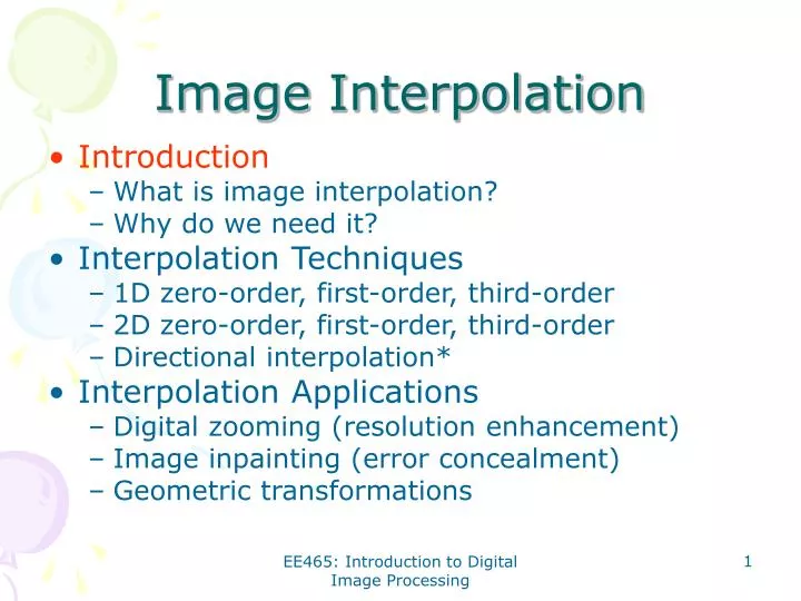
Image Interpolation • Introduction • What is image interpolation? • Why do we need it? • Interpolation Techniques • 1D zero-order, first-order, third-order • 2D zero-order, first-order, third-order • Directional interpolation* • Interpolation Applications • Digital zooming (resolution enhancement) • Image inpainting (error concealment) • Geometric transformations EE465: Introduction to Digital Image Processing
Introduction • What is image interpolation? • An image f(x,y) tells us the intensity values at the integral lattice locations, i.e., when x and y are both integers • Image interpolation refers to the “guess” of intensity values at missing locations, i.e., x and y can be arbitrary • Note that it is just a guess (Note that all sensors have finite sampling distance) EE465: Introduction to Digital Image Processing
Introduction (Con’t) • Why do we need image interpolation? • We want BIG images • When we see a video clip on a PC, we like to see it in the full screen mode • We want GOOD images • If some block of an image gets damaged during the transmission, we want to repair it • We want COOL images • Manipulate images digitally can render fancy artistic effects as we often see in movies EE465: Introduction to Digital Image Processing
Scenario I: Resolution Enhancement Low-Res. High-Res. EE465: Introduction to Digital Image Processing
Scenario II: Image Inpainting Non-damaged Damaged EE465: Introduction to Digital Image Processing
Scenario III: Image Warping EE465: Introduction to Digital Image Processing
Image Interpolation • Introduction • What is image interpolation? • Why do we need it? • Interpolation Techniques • 1D zero-order, first-order, third-order • 2D zero-order, first-order, third-order • Directional interpolation* • Interpolation Applications • Digital zooming (resolution enhancement) • Image inpainting (error concealment) • Geometric transformations EE465: Introduction to Digital Image Processing
1D Zero-order (Replication) f(n) n f(x) x EE465: Introduction to Digital Image Processing
1D First-order Interpolation (Linear) f(n) n f(x) x EE465: Introduction to Digital Image Processing
Linear Interpolation Formula Basic idea: the closer to a pixel, the higher weight is assigned f(n) f(n+a) f(n+1) a 1-a f(n+a)=(1-a)f(n)+af(n+1), 0<a<1 Note: when a=0.5, we simply have the average of two EE465: Introduction to Digital Image Processing
Numerical Examples f(n)=[0,120,180,120,0] Interpolate at 1/2-pixel f(x)=[0,60,120,150,180,150,120,60,0], x=n/2 Interpolate at 1/3-pixel f(x)=[0,20,40,60,80,100,120,130,140,150,160,170,180,…], x=n/6 EE465: Introduction to Digital Image Processing
1D Third-order Interpolation (Cubic) f(n) n f(x) x Cubic spline fitting EE465: Introduction to Digital Image Processing
From 1D to 2D • Just like separable 2D transform (filtering) that can be implemented by two sequential 1D transforms (filters) along row and column direction respectively, 2D interpolation can be decomposed into two sequential 1D interpolations. • The ordering does not matter (row-column = column-row) • Such separable implementation is not optimal but enjoys low computational complexity EE465: Introduction to Digital Image Processing
Graphical Interpretationof Interpolation at Half-pel row column f(m,n) g(m,n) EE465: Introduction to Digital Image Processing
Numerical Examples a b c d zero-order first-order a a b b a a b b c c d d c c d d a (a+b)/2 b (a+c)/2(a+b+c+d)/4 (b+d)/2 c (c+d)/2 d EE465: Introduction to Digital Image Processing
Numerical Examples (Con’t) Col n+1 Col n X(m,n) X(m,n+1) row m b a 1-a Y 1-b row m+1 X(m+1,n) X(m+1,n+1) Q: what is the interpolated value at Y? Ans.: (1-a)(1-b)X(m,n)+(1-a)bX(m+1,n) +a(1-b)X(m,n+1)+abX(m+1,n+1) EE465: Introduction to Digital Image Processing
Bicubic Interpolation* EE465: Introduction to Digital Image Processing
Edge blurring Jagged artifacts Limitation with bilinear/bicubic Jagged artifacts Edge blurring Z X Z X EE465: Introduction to Digital Image Processing
Directional Interpolation* Step 1: interpolate the missing pixels along the diagonal a b Since |a-c|=|b-d| x x has equal probability of being black or white c d black or white? Step 2: interpolate the other half missing pixels a Since |a-c|>|b-d| x d b x=(b+d)/2=black c EE465: Introduction to Digital Image Processing
Image Interpolation • Introduction • What is image interpolation? • Why do we need it? • Interpolation Techniques • 1D zero-order, first-order, third-order • 2D zero-order, first-order, third-order • Directional interpolation* • Interpolation Applications • Digital zooming (resolution enhancement) • Image inpainting (error concealment) • Geometric transformations EE465: Introduction to Digital Image Processing
Pixel Replication low-resolution image (100×100) high-resolution image (400×400) EE465: Introduction to Digital Image Processing
Bilinear Interpolation low-resolution image (100×100) high-resolution image (400×400) EE465: Introduction to Digital Image Processing
Bicubic Interpolation low-resolution image (100×100) high-resolution image (400×400) EE465: Introduction to Digital Image Processing
Edge-Directed Interpolation(Li&Orchard’2000) low-resolution image (100×100) high-resolution image (400×400) EE465: Introduction to Digital Image Processing
Image Demosaicing(Color-Filter-Array Interpolation) Bayer Pattern EE465: Introduction to Digital Image Processing
Image Example Advanced CFA Interpolation Ad-hoc CFA Interpolation EE465: Introduction to Digital Image Processing
Error Concealment damaged interpolated EE465: Introduction to Digital Image Processing
Image Inpainting EE465: Introduction to Digital Image Processing
Geometric Transformation Widely used in computer graphics to generate special effects MATLAB functions: griddata, interp2, maketform, imtransform EE465: Introduction to Digital Image Processing
Basic Principle • (x,y) (x’,y’) is a geometric transformation • We are given pixel values at (x,y) and want to interpolate the unknown values at (x’,y’) • Usually (x’,y’) are not integers and therefore we can use linear interpolation to guess their values MATLAB implementation: z’=interp2(x,y,z,x’,y’,method); EE465: Introduction to Digital Image Processing
Rotation y y’ x’ θ x EE465: Introduction to Digital Image Processing
MATLAB Example z=imread('cameraman.tif'); % original coordinates [x,y]=meshgrid(1:256,1:256); % new coordinates a=2; for i=1:256;for j=1:256; x1(i,j)=a*x(i,j); y1(i,j=y(i,j)/a; end;end % Do the interpolation z1=interp2(x,y,z,x1,y1,'cubic'); EE465: Introduction to Digital Image Processing
Rotation Example θ=3o EE465: Introduction to Digital Image Processing
Scale a=1/2 EE465: Introduction to Digital Image Processing
Affine Transform parallelogram square EE465: Introduction to Digital Image Processing
Affine Transform Example EE465: Introduction to Digital Image Processing
Shear parallelogram square EE465: Introduction to Digital Image Processing
Shear Example EE465: Introduction to Digital Image Processing
Projective Transform B’ B A A’ C’ D C D’ square quadrilateral EE465: Introduction to Digital Image Processing
Projective Transform Example [-4 2; -8 -3; -3 -5; 6 3] [ 0 0; 1 0; 1 1; 0 1] EE465: Introduction to Digital Image Processing
Polar Transform EE465: Introduction to Digital Image Processing
Iris Image Unwrapping r EE465: Introduction to Digital Image Processing
Use Your Imagination r -> sqrt(r) http://astronomy.swin.edu.au/~pbourke/projection/imagewarp/ EE465: Introduction to Digital Image Processing
Free Form Deformation Seung-Yong Lee et al., “Image Metamorphosis Using Snakes and Free-Form Deformations,”SIGGRAPH’1985, Pages 439-448 EE465: Introduction to Digital Image Processing
Application into Image Metamorphosis EE465: Introduction to Digital Image Processing
Summary of Image Interpolation • A fundamental tool in digital processing of images: bridging the continuous world and the discrete world • Wide applications from consumer electronics to biomedical imaging • Remains a hot topic after the IT bubbles break EE465: Introduction to Digital Image Processing