Download
1 / 21
3.82k likes | 11.02k Views
Email Spam Detection using machine Learning. Lydia Song, Lauren Steimle, Xiaoxiao Xu. Outline. Introduction to Project Pre-processing Dimensionality Reduction Brief discussion of different algorithms K-nearest D ecision tree Logistic regression Naïve-Bayes Preliminary results

E N D
Email Spam Detection using machine Learning Lydia Song, Lauren Steimle, XiaoxiaoXu
Outline • Introduction to Project • Pre-processing • Dimensionality Reduction • Brief discussion of different algorithms • K-nearest • Decision tree • Logistic regression • Naïve-Bayes • Preliminary results • Conclusion
Spam Statistics • Percentage of Spam Emails in email traffic averaged 69.9% in February 2014 Percentage of spam in email traffic Source: https://www.securelist.com/en/analysis/204792328/Spam_report_February_2014
Spam vs. Ham Spam=Unwanted communication Ham=Normal communication
Pre-processing Example of Spam Email Corresponding File in Data Set Spam Email in Web Browser
Pre-processing • Remove meaningless words • Create a “bag of words” used in data set • Combine similar words • Create a feature matrix “service” “last” “history” Email 1 Email 2 Email m
tokens= [‘your’, ‘history’, ‘shows’, ‘that’, ‘your’, ‘last’, ‘order’, ‘is’, ‘ready’, ‘for’, ‘refilling’, ‘thank’, ‘you’, ‘sam’, ‘mcfarland’, ‘customer services’] Pre-processing Example Your history shows that your last order is ready for refilling. Thank you, Sam Mcfarland Customer Services filtered_words=[ 'history', 'last', 'order', 'ready', 'refilling', 'thank', 'sam', 'mcfarland', 'customer', 'services'] “servi” “histori” “last” Email 1 bag of words=['history', 'last', 'order', 'ready', 'refill', 'thank', 'sam', 'mcfarland', 'custom', 'service'] Email 2 Email m
Dimensionality Growth • Add ~100-150 features for each additional email
Dimensionality Reduction • Add a requirement that words must appear in x% of all emails to be considered a feature
Dimensionality Reduction-Hashing Trick • Before Hashing: 70x9403 Dimensions • After Hashing: 70x1024 Dimensions String Integer Hash Table Index Source: Jorge Stolfi, http://en.wikipedia.org/wiki/File:Hash_table_5_0_1_1_1_1_1_LL.svg#filelinks
Outline • Introduction to Project • Pre-processing • Dimensionality Reduction • Brief discussion of different algorithms • K-nearest • Decision tree • Logistic regression • Naïve-Bayes • Preliminary results • Conclusion
K-Nearest Neighbors • Goal: Classify an unknown training sample into one of C classes • Idea: To determine the label of an unknown sample (x), look at x’s k-nearest neighbors Image from MIT Opencourseware
Decision Tree • Convert training data into a tree structure • Root node: the first decision node • Decision node: if–then decision based on features of training sample • Leaf Node: contains a class label Image from MIT Opencourseware
Logistic Regression • “Regression” over training examples • Transform continuous y to prediction of 1 or 0 using the standard logistic function • Predict spam if
Naïve Bayes • Use Bayes Theorem: • Hypothesis (H): spam or not spam • Event (e): word occurs • For example, the probability an email is spam when the word “free” is in the email • “Naïve”: assume the feature values are independent of each other
Outline • Introduction to Project • Pre-processing • Dimensionality Reduction • Brief discussion of different algorithms • K-nearest • Decision tree • Logistic regression • Naïve-Bayes • Preliminary results • Conclusion
Preliminary Results • 250 emails in training set, 50 in testing set • Use 15% as the “percentage of emails” cutoff • Performance measures: • Accuracy: % of predictions that were correct • Recall: % of spam emails that were predicted correctly • Precision: % of emails classified as spam that were actually spam • F-Score: weighted average of precision and recall
“Percentage of Emails” Performance Linear Regression Logistic Regression
Next Steps • Implement SVM: Matlab vs. Weka • Hashing trick- try different number of buckets • Regularizations