Download
1 / 34
340 likes | 596 Views
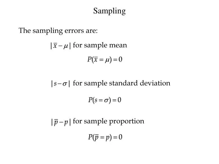
for sample mean. for sample standard deviation. for sample proportion. Sampling. The sampling errors are:. Sampling. Example: St. Andrew’s.

E N D
for sample mean for sample standard deviation for sample proportion Sampling The sampling errors are:
Sampling Example: St. Andrew’s St. Andrew’s College receives 900 applications annually from prospective students. The application form contains a variety of information including the individual’s scholastic aptitude test (SAT) score and whether or not the individual desires on-campus housing. • The director of admissions would like to know the following information: • Applicants’ average SAT score over the past 10 years • the proportion of applicants who live on campus.
Sampling Example: St. Andrew’s We will now look at two alternatives for obtaining the desired information. Conducting a census of all applicants over the last ten years (N = 9000) allows us to compute population parameters. Selecting a sample of 30 from the 9000 current applicants allows us to compute the sample statistics. If the relevant data for the entire 9000 applicants were in the college’s database, the population parameters of interest could be calculated using the formulas presented in Chapter 3.
Conducting a Census Population Mean SAT Score Population Proportion Wanting On-Campus Housing Population Standard Deviation for SAT Score
Conducting a Census m = 993
Conducting a Census Population Mean SAT Score Population Proportion Wanting On-Campus Housing Population Standard Deviation for SAT Score
Simple Random Sampling Suppose the data is stored in boxes off campus. The Director of Admissions needs estimates of the population parameters for a meeting taking place in an hour. She decides a sample of 30 applicants will be used. The number of random samples (without replacement) of size 30 that can be drawn from a population of size 9000 is huge. For just this year, it is
Simple Random Sampling Taking a Sample of 30 Applicants Step 1: Assign a random number to each of the 9000 current applicants. Excel’s RAND function generates random numbers between 0 and 1 Step 2: Select the 30 applicants corresponding to the 30 smallest random numbers.
Simple Random Sampling Sort rows by the random numbers
Simple Random Sampling 30 applicant numbers with smallest random numbers.
Simple Random Sampling Sample Mean SAT Score Sample Proportion Wanting On-Campus Housing Sample Standard Deviation for SAT Score
x = 1009.97 Simple Random Sampling
Simple Random Sampling Sample Mean SAT Score Sample Proportion Wanting On-Campus Housing Sample Standard Deviation for SAT Score
Sampling Distribution of E( ) = The sampling distribution of is the probability distribution of all possible values of the sample mean. Expected Value of where = the population mean Standard Deviation of from an infinite population is
Sampling Distribution of Under repeated sampling using random samples of size n, the sample means are normally distributed with mean m and variance s2/n when either The data is heavily skewed, n> 50, and sis known. OR The data is symmetric, n> 30, and sis known. OR The data is normally distributed and sis known.
Sampling Distribution of Sampling Distribution of
Sampling Distribution of What is the probability that a simple random sample of 30 applicants will provide an estimate of the population mean SAT score that is within 10 points of the actual population mean ? In other words, what is the probability that will be between 983 and 1003? Step 1: Calculate the z-value at the upper endpoint of the interval. z = (1003 - 993)/14.6 = .68
Sampling Distribution of Step 2: Find the area under the curve to the left of the upper endpoint. z = .68 P(x< 1003) = .7517 P(z< .68) = .7517
Sampling Distribution of Sampling Distribution of Area = .2483 Area = .7517 993 1003
Sampling Distribution of Step 3: Calculate the z-value at the lower endpoint of the interval. z = (983 - 993)/14.6 = - .68 Step 4: Find the area under the curve to the left of the lower endpoint. P(z< -.68) = .2483 P(x< 983) = .2483
Sampling Distribution of With n = 30, P(983 << 1003) = .5034 Step 5: Calculate the area under the curve between the lower and upper endpoints of the interval. .5034 .2483 .2483 983 993 1003
Sampling Distribution of E( ) remains equal to 993 With n = 30, If the simple had included 100 applicants instead of 30, , but the standard error falls. .5034 .2483 .2483 983 993 1003
Sampling Distribution of E( ) remains equal to 993 With n = 30, If the simple had included 100 applicants instead of 30, , but the standard error falls. With n = 100, .7888 .5034 .2483 .2483 983 993 1003
The sampling distribution of is approximately normal when Sampling Distribution of The Expected value of Standard deviation of from an infinite population is sD = standard deviation of D np> 5 n(1 – p) > 5 and
Sampling Distribution of The sample proportion can be computed in the same way as the sample mean when a dummy variable is coded from a nominal scaled binomial variable.
Sampling Distribution of The sampling distribution of is the probability distribution of all possible values of the sample proportion. We should have divided by n – 1 because the data came from a sample. Since there are six1s and four0s In most cases involving sample proportions, n is very large. Hence, dividing by n or n – 1 yields roughly the same value
Sampling Distribution of Example: St. Andrew’s College Recall that 72% of the prospective students applying to St. Andrew’s College desire on-campus housing. What is the probability that a simple random sample of 30 applicants will provide an estimate of the population proportion of applicants desiring on-campus housing that is within .05 of the actual population proportion? Step 1: Convert the upperendpoint of the interval to z. P(0.67 <<0.77) = ? z1= (.77 - .72)/.082 = .61
Sampling Distribution of For this example, with n = 30 and p = .72, the normal distribution is an acceptable approximation because: and n(1 - p) = 30(.28) = 8.4 > 5 np = 30(.72) = 21.6 > 5 ? .72 .77 .67
Sampling Distribution of Step 2: Find the area under the curve to the right of the upper endpoint. z1= .61 P(z1< .61) = .7291 P(p< .77) = .7291
Sampling Distribution of Area = .2709 Area = .7291 .72 .77
Sampling Distribution of Step 3: Calculate the z-value of the lower endpoint of the interval. z0= (.67 - .72)/.082 = -.61 Step 4: Find the area under the curve to the left of the lower endpoint. P(z0< -.61) = .2709 P(p< .67) = .2709
Sampling Distribution of Step 5: Calculate the area under the curve between the lower and upper endpoints of the interval. Area = .2709 Area = .2709 .4582 .77 .67 .72
= Sample mean SAT score = Sample pro- portion wanting campus housing Simple Random Sampling Population Parameter Parameter Value Point Estimator Point Estimate m = Population mean SAT score 1009.97 993 s = Sample std. deviation for SAT score s= Population std. deviation for SAT score 80 85.45 p = Population pro- portion wanting campus housing .72 .667