Environmental Economics: Lecture 7

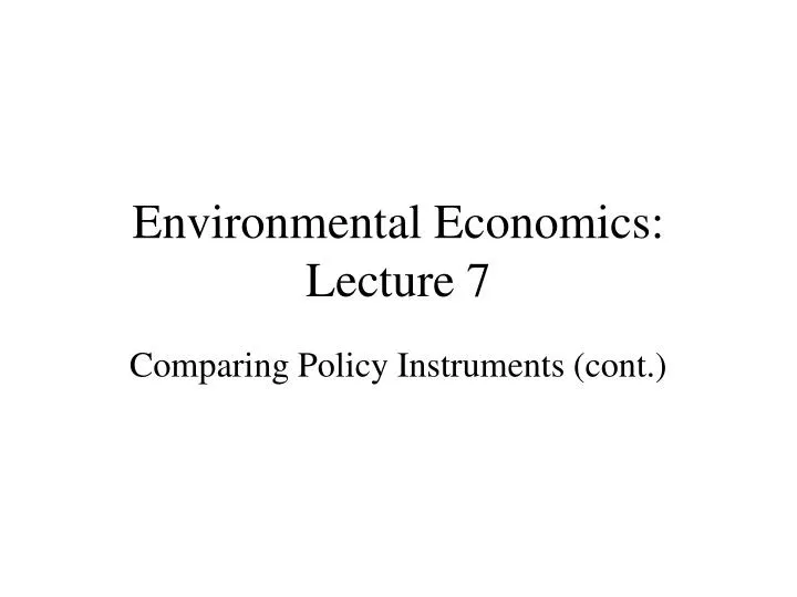
Environmental Economics: Lecture 7 Comparing Policy Instruments (cont.)

Outline • Review 3 graphs & basic tools • Key results so far • New areas • Midnight Dumping • Innovation • Areas not addressed in our survey so far

Our model so far: graph #1 Price and Cost Equilibrium Price PA MPC (supply curve) Quantity MSC= MPC+MED MED (externality) D= Marginal SocialBenefit

Basic Tools • When changing quantity, we focus on areas under curves • Below MB = Change in benefits • Below MC = Change in costs • Below MED = Area between SMC & MPC = change in externality • With perfect competition, P=MR=MPC, which determines the “competitive output.” • With perfect competition, area below MB, but above price = consumer’s surplus

Equilibrium with a Negative Externality Price and Cost MSC B MPC (supply curve) A Equilibrium Price PA D= Marginal SocialBenefit 8,000 Units 10,000 Units Quantity Economically Efficient Output Equilibrium Output

Result #1: inefficiency of externality • We used graph #1 to identify the costs of moving from “competitive equilibrium quantity”, to “socially optimal quantity.” • Specifically we compared • Lost benefits (below MB), to: • Private cost savings (below PMC) & Reductions in Externality (below MED=between PMC & MED). • Result: Reduction in costs (both types) is greater than reduction in ben. • Implication: competitive market inefficient (dead-weight loss).

Economic Inefficiency with a Negative Externality P MSC $180 Deadweight Social Loss MPC = S PA = $100 D Q 10,000 Units Equilibrium Output

Result #2: Coase theorem • Considered case where MB and MED both affect only a small number of people. • Argued that if we assign “rights to pollute” there would be substantial incentives to negotiate a side payment that results in efficient level.Two scenarios • Bart compensates Lisa (who has the right to prevent pollution). • Lisa “bribes” Bart to pollute less (even though he has the right)

List of Policy Instruments • As a class, we developed a full list of potential policies a government could use to correct an externality. • In order to compare instruments, we need to move beyond some of the limitations implicit in graph #1.

Limitations of Graph #1 • Has output on the horizontal axis. • Implication: the only way to reduce pollution is to reduce output. • Extension: Graph #2 (Fullerton, SEJ) uses pollution (not output) on horizontal axis • Has a single MC curve for the entire industry. • Implication: all firms are the same. • Extension: Graph #3 models the marginal cost of abatement (pollution reduction) faced by firms. Graph allows MAC to differ by firm.

Graph #2 • Pollution on horizontal axis (assumes perfect competition) • Here, “price” implies the price associated with the polluting input. • The consumer’s total price (and CS) is in some sense the sum of prices associated with each input. • Reducing pollution might mean reducing output, or changing inputs, or doing filtration, etc. • Any of these raises price and reduces consumer’s surplus associated with the final good or service.

Result #3 • A variety of instruments that each achieve the efficient level of pollution have very different distributional consequences.

Graph #3 (version a): marginal abatement costs • Instead of looking at the decision about how much to pollute, the graph looks at the decision to reduce pollution relative to some “baseline” amount. • Abatement = negative pollution • If graph includes the marginal benefit of abatement we can identify an optimal level of abatement (version b). • In our first version of this graph, we simply depicted two firms with two different MAC curves (version a).

Result #4: CAC/performance standard is inefficient • A command and control policy requiring uniform abatement levels is inefficient when firms have differing marginal costs. • On graph, specify some point, A, that each firm has to abate. • On graph, find the additional costs to low marginal cost firm of abating a little more. • On graph, find the savings to high marginal cost firm of abating a little less. • If savings > additional costs, uniform policy is inefficient. • Caveat: result requires “perfect mixing”

Result #5: Efficiency of incentive-based instruments • a tradable permit system or Pigouvian tax (emission fee) is efficient. • To show for permits, start again at point where firms do uniform level of abatement. • Consider their incentives to buy and sell rights to pollute. • Argue that pareto-improvements are possible. • Identify the point at which the price at which the high cost firm is willing buy permits equals the price at which the low-cost firm is willing to sell permits. • At this allocation, no pareto improvements are possible. • For taxes, start with a tax set at the price identified above. • Identify the point at which each firm prefers to pay the tax, rather than abate. • Show that it produces same allocation as permits (no Pareto improvements possible)

Graph #3, version b • Choice of policy instruments under uncertainty. • Here we again assume a single Marginal abatement cost curve, but add MB of abatement. • Also add uncertainty.

Uncertainty in Marginal Costs • Case 1 (MC steep, MB flat) • In this case, taxes lead to smaller dead-weight loss.

Graph 3b, case 1 MACAct Cost MACEx MB Abatement

Steps to finding DWL • Find the Q* (optimal quantity) • Find the Qact (Abatement actually produced) • For the area between Qact and Q* find how much costs exceed benefits. • These steps are simpler for permit than for tax.

Graph 3b, case 1 with Q-instrument MACAct Cost MACEx MB Qact Q* Abatement

Graph 3b, case 1 with tax MACAct Cost MACEx tax MB Abatement

Graph 3b, case 1 with tax MACAct Cost MACEx tax MB Q* Abatement Qactual

Graph 3b, comparing instruments MACAct Cost MACEx MB Abatement

Environmental Economics: Lecture 7