Download
1 / 20
200 likes | 314 Views
Simple stochastic models 2. Continuous random variable X. X – can take values: - < x < + Cumulative probability distribution function: P X (x) = P(X x) Probability density function:. Normal distribution. X ~ normal( ,), E(X)= , V(X)= 2. pdf:. cpdf:.

E N D
Continuous random variable X X – can take values: - < x < + Cumulative probability distribution function: PX(x) = P(X x) Probability density function:
Normal distribution X ~ normal(,), E(X)= , V(X)= 2 pdf: cpdf:
=0, =1 0.4 0.3 pdf 0.2 0.1 0 -4 -3 -2 -1 0 1 2 3 4 cpdf x
Central limit theorem Y = X1 + X2 + … +Xn Xi - independent, zero mean, equal varianceV If n is large then: ~ normal(0,1)
0.07 0.06 0.05 0.04 0.03 0.02 0.01 0 Example – students body heights Histogram of students’ body heights versus normal probability density function 160 165 170 175 180 185 190 195 200 205
9 8 7 6 5 4 3 2 1 0 Example – children birth weights Histogram of children birth weights versus normal probability density function -4 x 10 0 1000 2000 3000 4000 5000 6000
Binomial becomes normal 0.12 0.1 0.08 0.06 0.04 0.02 0 0 5 10 15 20 25 30 35 40 45 50 o – binomial(0.5,50) normal(25,3.5355)
How do we fit normal distribution to data ? Data: X1, X2, …, Xn
How do we estimate parameters of distributions using data ? • How do we verify that data follow a given distribution ?
Characteristic function X – with pdf p(x) characteristic function:
Properties Y=aX+b, a,b - constants
Characteristic function of normal distribution X ~ normal(,),
Two dimensional distributions X, Y Probability density function: p(x,y) Cumulative pdf:
Independent random variables X, Y independent pXY(x,y)=pX(x) pY(y) Convolution integral Z=X+Y pZ = pX * pY
Use of characteristic functions to prove Central Limit Theorem Y = X1 + X2 + … +Xn i=1,2…,n so: and