Download
1 / 28
280 likes | 325 Views
This article discusses covering algorithms in classification, focusing on generating rule sets for each class, PRISM algorithm, nearest-neighbor techniques, instance-based classification, and distance functions. It also covers topics like normalization, k-NN approaches, and dealing with noisy data. The text provides insights into the strategies and challenges of generating rules and making accurate predictions in machine learning.

E N D
Classification Algorithms • Covering, Nearest-Neighbour
Covering algorithms • Strategy for generating a rule set directly: • for each class in turn find rule set that covers all examples in it (excluding examples not in the class) • This approach is called a covering approach • at each stage a rule is identified that covers some of the examples
entire dataset Example: generating a rule
Example: generating a rule a single rule describes a convex concept
Example: generating a rule • ‘b’ is not convex need extra rules for else part • possible rule set for class ‘b’ • more rules could be added for a ‘perfect’ rule set
Rules vs. Trees • Corresponding decision tree: (produces exactly the same predictions)
A simple covering algorithm: PRISM • Generate a rule by adding tests that maximize a rule’s accuracy • Each additional test reduces a rule’s coverage:
Selecting a test • Goal: maximize accuracy • t total number of examples covered by rule • p positive examples of the class covered by rule • Select test that maximizes the ratio p/t • We are finished when p/t= 1 or the set of examples cannot be split any further
Example: contact lens data • Rule we seek: • Possible tests:
Modified rule and resulting data • Rule with best test added (4/12): • Examples covered by modified rule:
Further refinement • Current state: • Possible tests:
Modified rule and resulting data • Rule with best test added: • Examples covered by modified rule:
Further refinement • Current state: • Possible tests: • Tie between the first and the fourth test • We choose the one with greater coverage
The result • Final rule: • Second rule for recommending “hard” lenses:(built from examples not covered by first rule) • These two rules cover all “hard”lenses • Process is repeated with other two classes
Separate and conquer • Methods like PRISM (for dealing with one class) are separate-and-conqueralgorithms: • First, a rule is identified • Then, all examples covered by the rule are separated out • Finally, the remaining examples are “conquered” • Difference to divide-and-conquer methods: • Subset covered by rule doesn’t need to be explored any further
Instance-based Classification k-nearest neighbours
Instance-based representation • Simplest form of learning: rote learning • Training set is searched for example that most closely resembles new example • The examples themselves represent the knowledge • Also called instance-based learning • Instance-based learning is lazy learning • Similarity function defines what’s “learned” • Methods: • nearest neighbour • k-nearest neighbours • …
The distance function • Simplest case: one numeric attribute • Distance is the difference between the two attribute values involved (or a function thereof) • Several numeric attributes: normally, Euclidean distance is used and attributes are normalized • Are all attributes equally important? • Weighting the attributes might be necessary
The distance function • Most instance-based schemes use Euclidean distance: a(1) and a(2): two instances with k attributes • Taking the square root is not required when comparing distances • Other popular metric: city-block (Manhattan) metric • Adds differences without squaring them
Normalization and other issues • Different attributes are measured on different scales • Need to be normalized: vi: the actual value of attribute i • Nominal attributes: distance either 0 or 1 • Common policy for missing values: assumed to be maximally distant (given normalized attributes) or
k-NN example • k-NN approach: perform a majority vote to derive label
Discussion of 1-NN • Can be very accurate • But: curse of dimensionality • Every added dimension increases distances • Exponentially more training data needed • … but slow: • simple version scans entire training data to make prediction • better training set representations: kD-tree, ball tree,... • Assumes all attributes are equally important • Remedy: attribute selection or weights • Possible remedy against noisy examples: • Take a majority vote over the k nearest neighbours
Summary • Simple methods frequently work well • robust against noise, errors • Advanced methods, if properly used, can improve on simple methods • No method is universally best