Download
1 / 38
390 likes | 633 Views
4.3 NORMAL PROBABILITY DISTRIBUTIONS. The Most Important Probability Distribution in Statistics. Normal Distributions . A random variable X with mean m and standard deviation s is normally distributed if its probability density function is given by. The Shape of Normal Distributions.

E N D
4.3 NORMAL PROBABILITY DISTRIBUTIONS The Most Important Probability Distribution in Statistics
Normal Distributions • A random variable X with mean m and standard deviation sis normally distributed if its probability density function is given by
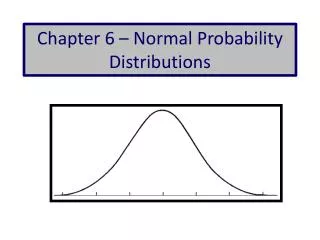
The Shape of Normal Distributions Normal distributions are bell shaped, and symmetrical around m. m 90 110 Why symmetrical? Let m = 100. Suppose x = 110. Now suppose x = 90
Normal Probability Distributions • The expected value (also called the mean) E(X) (or )can be any number • The standard deviation can be any nonnegative number • The total area under every normal curve is 1 • There are infinitely many normal distributions
The effects of m and s How does the standard deviation affect the shape of f(x)? s= 2 s =3 s =4 How does the expected value affect the location of f(x)? m = 10 m = 11 m = 12
X 0 3 6 9 12 8 µ = 3 and = 1 A family of bell-shaped curves that differ only in their means and standard deviations. µ = the mean of the distribution = the standard deviation
µ = 3 and = 1 X 0 3 6 9 12 µ = 6 and = 1 X 0 3 6 9 12
X 0 3 6 9 12 8 X 0 3 6 9 12 8 µ = 6 and = 2 µ = 6 and = 1
Probability = area under the density curve P(6 < X < 8) = area under the density curve between 6 and 8. a b a b X µ = 6 and = 2 P(6 < X < 8) X 0 3 6 9 12
Probability = area under the density curve P(6< X <8) = area under the density curve between 6 and 8. a b a b X µ = 6 and = 2 P(6 < X < 8) X 0 3 6 9 12 8 6 8 6 8
Probability = area under the density curve P(6< X <8) = area under the density curve between 6 and 8. a b a b X 6 8 6 8
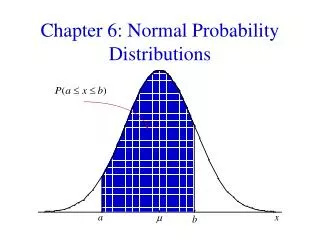
P(a < X < b) f(x) Probabilities: area under graph of f(x) X a b P(a < X < b) = area under the density curve between a and b. P(X=a) = 0 P(a < x < b) = P(a < x < b)
Standardizing • Suppose X~N( • Form a newrandom variable by subtracting the mean from X and dividing by the standard deviation : (X • This process is called standardizing the random variable X.
Standardizing (cont.) • (X is also a normal random variable; we will denote it by Z: Z = (X • has mean 0 and standard deviation 1:E(Z) = = 0; SD(Z) = = 1. • The probability distribution of Z is called the standard normal distribution.
Standardizing (cont.) • If X has mean and stand. dev. , standardizing a particular value of x tells how many standard deviations x is above or below the mean . • Exam 1: =80, =10; exam 1 score: 92 Exam 2: =80, =8; exam 2 score: 90 Which score is better?
X 0 3 6 9 12 .5 .5 8 (X-6)/2 Z -3 -2 -1 0 1 2 3 µ = 6 and = 2 µ = 0 and = 1
Pdf of a standard normal rv • A normal random variable x has the following pdf:
.5 .5 Z -3 -2 -1 0 1 2 3 Standard Normal Distribution Z = standard normal random variable = 0 and = 1 .5 .5
Important Properties of Z #1. The standard normal curve is symmetric around the mean 0 #2. The total area under the curve is 1; so (from #1) the area to the left of 0 is 1/2, and the area to the right of 0 is 1/2
Finding Normal Percentiles by Hand (cont.) • Table Z is the standard Normal table. We have to convert our data to z-scores before using the table. • The figure shows us how to find the area to the left when we have a z-score of 1.80:
.1587 Z Areas Under the Z Curve: Using the Table P(0 < Z < 1) = .8413 - .5 = .3413 .50 .3413 0 1
P(- <Z<z0) Standard normal probabilities have been calculated and are provided in table Z. The tabulated probabilities correspond to the area between Z= - and some z0 Z = z0
Example – continued X~N(60, 8) 0.8944 0.8944 0.8944 0.8944 = 0.8944 0.8944 0.8944 P(z < 1.25) In this example z0 = 1.25
Area=.3980 z 0 1.27 Examples • P(0 z 1.27) = .8980-.5=.3980
A2 0 .55 P(Z .55) = A1 = 1 - A2 = 1 - .7088 = .2912
z 0 -2.24 Examples Area=.4875 • P(-2.24 z 0) = Area=.0125 .5 - .0125 = .4875
.1190 Examples (cont.) • P(-1.18 z 2.73) = A - A1 • = .9968 - .1190 • = .8778 .9968 A1 A2 A A1 z -1.18 0 2.73
P(-1 ≤ Z ≤ 1) = .8413 - .1587 =.6826 vi) P(-1≤ Z ≤ 1) .6826 .1587 .8413
6. P(z < k) = .2514 6. P(z < k) = .2514 .5 .5 -.67 .2514 Is k positive or negative? Direction of inequality; magnitude of probability Look up .2514 in body of table; corresponding entry is -.67
Examples (cont.) viii) .7190 .2810
Examples (cont.) ix) .8671 .1230 .9901
.1587 Z P( Z < 2.16) = .9846 .9846 Area=.5 .4846 0 2.16
Example • Regulate blue dye for mixing paint; machine can be set to discharge an average of ml./can of paint. • Amount discharged: N(, .4 ml). If more than 6 ml. discharged into paint can, shade of blue is unacceptable. • Determine the setting so that only 1% of the cans of paint will be unacceptable