Download
1 / 75
750 likes | 947 Views
KVANLI PAVUR KEELING. Chapter 3 Data Summary Using Descriptive Measures. Chapter Objectives. At the completion of this chapter, you should be able to define and use the following measures: ∙ Measures of Central Tendency: Mean, Median, Mode and Midrange

E N D
KVANLI PAVUR KEELING Chapter 3Data Summary Using Descriptive Measures
Chapter Objectives • At the completion of this chapter, you should be able to define and use the following measures: ∙ Measures of Central Tendency: Mean, Median, Mode and Midrange ∙ Measures of Variation: Range, Standard Deviation, Variance, and Coefficient of Variation
Chapter Objectives - Continued • At the completion of this chapter, you should be able to define and use the following measures: ∙ Measures of Position: Percentiles, Quartiles, and z-scores ∙ Measures of Shape: Skewness and Kurtosis
Summarizing a Sample • Chapter 2 described a sample using a graph or chart • This chapter summarizes a sample by crunching a number or two, such as an average • We refer to these number as descriptivemeasures • There are four different types of descriptive measures
Descriptive Measures • There are measures of: • central tendency • variation • position • shape • Consider a sample consisting of the number of purchased textbooks this semester for 5 randomly selected students • The sample values are {6, 9, 7, 23, 5} Here, the sample size is n = 5
Measures of Central Tendency • These are: • mean • median • midrange • mode These determine where the “middle” of the sample is; that is, a “typical” value The mode is that value that occurs the most often
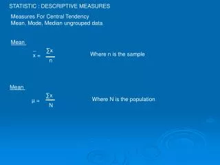
The Sample Mean • The sample mean is the sample average • Our sample: {6, 9, 7, 23, 5} • The sample mean is books • The symbol for the sample mean is • So, = 10 Read as “x bar”
The Sample Median • To find the median, you must first put the values in order from smallest to largest • For our sample, this would be {5, 6, 7, 9, 23} • When n is odd, the median is the value in the middle of the ordered data • The symbol for the median is Md • Here, Md = 7 • In general for n odd, Md is the value Here, this would be the 3rd value
The Sample Median – n is Even • Consider this sample: {2, 4, 8, 12, 16, 18} (n = 6) • When n is even, the median is the average of the middle two values • Here, Md = books • In general for n even, Md is the average of the value and the next one
The Sample Midrange • The midrange is the average of lowest (L) and highest (H) sample values • The symbol for the midrange is Mr • Mr= • The textbook sample is {6, 9, 7, 23, 5} • Here, Mr = This is H This is L
The Sample Mode • The mode is that value that occurs the most often in the sample • For the textbook example, there is no mode since there are no repeat values • If there is a 2-way tie, you state that the modes are ____ and ____ • For continuous data, don’t bother looking for a mode
More on the Sample Mode • If your company manufactures clothing, the sample mode is more likely to be of interest rather than the other three measures of central tendency • Example: You company manufactures hats • The statistic of interest in a sample of head sizes would be the most popular head size since we should manufacture more hats of that size • The mean (say, 6.82) would be of little interest • Ditto for the median and midrange
Choosing between the mean, median, and midrange • Consider the textbook sample {5, 6, 7, 9, 23} • The value of 23 is called an outlier since it is unusually large and doesn’t fit with the other four values • When trying to determine the middle (a “typical value”), which of these three measures of central tendency were most affected by this outlier?
The Effect of an Outlier • This outlier had the biggest impact on the midrange • Its value is 14, which exceeds 4 of the 5 sample values • This outlier also had a big impact on the mean • Its value is 10, which also exceeds 4 of the 5 sample values • But the outlier had NO effect on the sample median
Outliers and the Median • To illustrate this, suppose the sample values are {5, 6, 7, 9, 2300} • The midrange and mean are considerably larger than before • But the sample median is still 7 • It didn’t even change!
Moral to the Story • If you expect (or know) your sample contains outliers, use the median. Otherwise, use the mean. • Examples Incomes usually contain a few very large values. Use the median. House prices in a particular neighborhood typically contain a few very large values. Use the median.
Calculators • Most any calculator will work in this course. • If you prefer to use the TI-83 or TI-86, there are links on the DSCI 2710 website that show you how to crunch numbers on these two calculators. • If you’re going to purchase a calculator, I’d recommend the TI BA II Plus. It works very well in this course and is easy to use.
Measures of Variation • These are: • range (R) • variance (s2) • standard deviation (s) • coefficient of variation (CV) The most popular
The Sample Range (R) • The range is the difference of the highest and lowest sample values • R = H – L • Textbook sample: {5, 6, 7, 9, 23} • R = 23 – 5 = 18 • The sample range is a good measure of variation (and easy to compute) for small samples ( n ≤ 10)
The Sample Variance x 5 5 – 10 = -5 25 6 6 – 10 = -4 16 7 7 – 10 = -3 9 9 9 – 10 = -1 1 23 23 – 10 = 13169 0 220 Always is
The Sample Variance • The sum of the squared deviations (220) is then divided by n – 1 (not the sample size (n) as you might expect) • This is the sample variance (s2) • s2 = • In general, s2 =
The Sample Standard Deviation • The sample standard deviation (s) is the square root of the variance • s = • Here, s = • The units on the standard deviation are the same as the units on the sample data • For this example, s = 7.416 books
Using a Calculator • When deriving the standard deviation, we first found the variance and then found the square root of this value • When using a calculator, you reverse this sequence by ∙ entering the sample values ∙ hit the standard deviation key ∙ if you want a variance, hit the x2 key This is the way to do it!
The Sample Coefficient of Variation • The coefficient of variation (CV) is useful for comparing variation in two or more samples • Consider the following two samples: Sample #1 {5, 6, 7, 9, 23} the textbook sample Sample #2 {500, 600, 700, 900, 2300} • Question: Which sample has more variation?
The Sample Coefficient of Variation • For sample #1: x = 10 and s = 7.416 • For sample #2, it turns out that the previous mean and standard deviation are simply multiplied by 100; that is, x = 1000 and s = 741.6 • If you compared the two standard deviations, you might conclude that sample #2 has more variation • But, these sample values are simply larger
The Sample Coefficient of Variation • In fact, relative to the mean, the variation in these two samples is the same • To effectively compare the variation in these two samples, you should compute the coefficient of variation (CV) for each sample, where CV = · 100
The Sample Coefficient of Variation • For sample #1, CV = · 100 = 74.16 • For sample #2, CV = · 100 = 74.16 • For both samples, the standard deviation is 74.16% of the mean • MORAL: Don’t compare sample standard deviations unless the sample means are about the same
Describing a Population • Populations also have a mean, variance, and standard deviation Population (size is N) The population mean is μ (mu, pronounced “myoo”) and the population standard deviation is σ (sigma) The sample mean is and the sample standard deviation is s Sample (size is n)
The Dreaded Formulas Sample Population You divide by N (not N-1) σ2 is the population variance
Measures of Position • Measures of position include • Percentiles ∙ Special percentiles • z-scores These are called quartiles
Percentiles • Consider the 50 aptitude test scores introduced in Chapter 2 These values must be sorted Table 3.2
Percentiles • There are two rules to apply here • What is the 35th percentile? This uses Rule #1 • To find: 50 · .35 = 17.5 • Rule #1: Round this product up (always up) • So, the 35th percentile is the 18th value in the ordered array Rule #1 applies when this is not a counting number
Percentiles • What is the 60th percentile? This uses Rule #2 • To find: 50 · .60 = 30 • Rule #2: The percentile is the average of this value (the 30th value) and the next one (the 31st value) Rule #2 applies when this is a counting number
Quartiles • These are special percentiles • There are three quartiles (Q1, Q2, and Q3) • Q1 is the 25th percentile • Q2 is the 50th percentile • Q3 is the 75th percentile
Quartiles • Using the 50 aptitude scores, determine Q1 • This is the 25th percentile: 50 · .25 = 12.5 • So, Q1 is the 13th value in the ordered array • This value is 46 Not a counting number. So, use Rule #1
Quartiles • Q2 is the 50th percentile: 50 · .50 = 25 • Q2 is the average of the 25th and the 26th values in the ordered array • Q2 = (61 + 63)/2 = 62 • This is also the sample median • These two rules guarantee that Q2 is always equal to the sample median (and the 50th percentile) This is a counting number. So, use Rule #2
Quartiles • Q3 is the 75th percentile: 50 · .75 = 37.5 • So, Q3 is the 38th value in the ordered array • This value is 75 Not a counting number. So, use Rule #1 It was just a fluke that the 75th percentile was equal to 75
Another Measure of Position • A z-score is another measure of position • Every value in your sample has a corresponding z-score • How to find: z-score = where x is the sample value, x is the sample mean, and s is the sample standard deviation • The value of a z-score is how many standard deviations that sample value is to the left or right of the sample mean
Finding a z-score =60.36 s = 18.61
Finding a z-score • The corresponding z-score is • 90 is 1.59 standard deviations to the right of the mean • A z-score is positive if the sample value lies to the right of the mean and is negative if the sample value lies to the left of the mean • Typically, about half the z-scores will be positive and about half will be negative
Interpreting a z-score • These results are usually true Your z-score is 2.3 Approx. 68% z-score -3 -2 -1 0 1 2 3 Approx. 95% Nearly all
Interpreting a z-score - Assumptions • The previous slide is called the Empirical Rule • This rule assumes that the population from which you got the sample is bell-shaped • This means that if you were able to get the entire population and make a histogram of it, it would resemble the histogram on the next slide. • This is generally (approximately) true – but not always
Another Measure of Variation • The interquartile range (IQR) is another measure of variation and is the difference of the third and first quartiles • IQR = Q3 – Q1 • In the aptitude test scores, Q3 = 75 (the 75th percentile) and Q1= 46 (the 25th percentile) • IQR = 75 – 46 = 29 and so the middle 50% of the sample values cover a range of 29 • The larger this is, the more variation there is in the sample data
Measures of Shape • There are two measures in this category • skewness – A measure of the symmetry in the sample values (histogram) • kurtosis – A measure of how peaked the sample histogram is
Kurtosis • We’ll give this a very light treatment (no formulas). These two histograms illustrate high and low kurtosis High kurtosis – very peaked Low kurtosis – very flat
Skewness • Pearson’s measure of skewness Sk = ∙ Ranges from -3 to 3 ∙ Not the formula Excel uses • The next three slides demonstrate what Sk tells you about the shape of the histogram Subtract the mean and median, multiply by 3, and divide by the standard deviation
Frequency x = Md Histogram of Symmetric Data Sk ≈ 0 Figure 3.6