Download
1 / 14
140 likes | 270 Views
Development of an object-oriented verification technique for QPF. Michael Baldwin 1 Matthew Wandishin 2 , S. Lakshmivarahan 3 1 Cooperative Institute for Mesoscale Meteorological Studies, University of Oklahoma 2 Institute for Atmospheric Physics, University of Arizona

E N D
Development of an object-oriented verification technique for QPF Michael Baldwin1 Matthew Wandishin2, S. Lakshmivarahan3 1 Cooperative Institute for Mesoscale Meteorological Studies, University of Oklahoma 2 Institute for Atmospheric Physics, University of Arizona 3 School of Computer Science, University of Oklahoma
Traditional verification • Compare a collection of matching pairs of forecast and observed values at the same set of points in space/time • One “score” might end up representing the accuracy of millions of points, thousands of cases, hundreds of meteorological events • Boiling down that much information into a couple of numbers is not very meaningful
OBSERVED FCST #1: smooth Forecast #1: smooth OBSERVED FCST #2: detailed
“Measures-oriented” (Brooks and Doswell, 1996) approach to verifying these forecasts
Characterize the forecast and observed fields • Verify the forecast with a similar approach that a human forecaster would use to visualize the forecast/observed fields • Characterize features, phenomena, events, etc. found in forecast and observed fields by assigning attributes to each object
Object-oriented approach to verification • Decompose fields into sets of objects that can be objectively identified and described by attributes • Use image processing and data mining techniques to locate and classify events • Produce scores based upon the similarity/dissimilarity between forecast and observed objects • Analyze joint distribution of forecast and observed objects • Similar to Neilley (1993)
Possible scores produced by this approach d f f = (af, bf, cf, …, xf, yf ) o = (ao, bo, co, …, xo, yo) • score = function( f , o) • d ( f , o ) = ( f - o )t A ( f - o ) Generalized Euclidean distance, measure of dissimilarity A is a weight matrix, different attributes would probably have different weights • c ( f , o ) = cov ( f , o ) Covariance, measure of similarity o
Event #16 Characterization: How? • Locate an event Could use image processing edge detection routines
Characterization: How? • Assign attributes Examples: location, mean, variance, structure Event #16 x=37.3, y=87.8, b=2.8
attribute? Multiscale statistical properties (Harris et al 2001) • Fourier power spectrum • Generalized structure function: spatial correlation • Moment-scale analysis: intermittency of a field, sparseness of sharp intensities • Looking for “power law”, much like in atmospheric turbulence (–5/3 slope) FIG. 3. Isotropic spatial Fourier power spectral density (PSD) for forecast RLW (qr; dotted line) and radar-observed qr (solid line). Comparison of the spectra shows reasonable agreement at scales larger than 15 km. For scales smaller than 15 km, the forecast shows a rapid falloff in variability in comparison with the radar. The estimated spectral slope with fit uncertainty is = 3.0 ± 0.1
Fourier power spectra • Compare 3h accumulated QPF to radar/gage analyses • Forecasts were linearly interpolated to same 4km grid as “Stage IV” analysis • Errico (1985) Fourier analysis code used. 2-d Fourier transform converted to 1-d by annular average • Fixed grid used for analysis located away from complex terrain of Western U.S. • Want to focus on features generated by model physics and dynamics, free from influence of orographically forced circulations
Example Obs_4 Eta_12 Eta_8 log[E(k)] log[wavenumber] WRF_22 WRF_10 KF_22
Summary • Developing an “object-oriented” verification approach by characterizing forecasts and observations • Examining use of spatial structure and variability as potential attributes • Provides information on realism of forecasts that traditional QPF verification measures do not • Working with forecasters/users to determine useful attributes for characterizing events