Download
1 / 64
680 likes | 1.23k Views
Hyperbolic Processes in Finance. Alternative Models for Asset Prices. Outline. The Black-Scholes Model Fit of the BS Model to Empirical Data Hyperbolic Distribution Hyperbolic Lévy Motion Hyperbolic Model of the Financial Market Equivalent Martingale Measure

E N D
Hyperbolic Processes in Finance Alternative Models for Asset Prices Maria Adler University of Kaiserslautern Department of Mathematics
Outline • The Black-Scholes Model • Fit of the BS Model to Empirical Data • Hyperbolic Distribution • Hyperbolic Lévy Motion • Hyperbolic Model of the Financial Market • Equivalent Martingale Measure • Option Pricing in the Hyperbolic Model • Fit of the Hyperbolic Model to Empirical Data • Conclusion
The Black-Scholes Model price process of a security described by the SDE volatility drift Brownian motion price process of a risk-free bond interest rate
The Black-Scholes Model • Brownian motion has continuous paths • stationary and independent increments • market in this model is complete • allows duplication of the cash flow of • derivative securities and pricing by • arbitrage principle
Fit of the BS Model to Empirical Data • statistical analysis of daily stock-price data from 10 of the DAX30 companies • time period: 2 Oct 1989 – 30 Sep 1992 (3 years) • 745 data points each for the returns • Result: assumption of Normal distribution underlying the • Black- Scholes model does not provide a good fit to • the market data
Fit of the BS Model to Empirical Data Quantile-Quantile plots & density-plots for the returns of BASF and Deutsche Bank to test goodness of fit: Fig. 4, E./K., p.7
Fit of the BS Model to Empirical Data BASF Deutsche Bank
Fit of the BS Model to Empirical Data • Brownian motion represents the net random effect of the various factors of influence in the economic environment • (shocks; price-sensitive information) • actually, one would expect this effect to be discontinuous, as the individual shocks arrive • indeed, price processes are discontinuous looked at closely enough (discrete ´shocks´)
Fit of the BS Model to Empirical Data • Fig. 1, E./K., p.4 • typical path of a Brownian motion • continuous • the qualitative picture does not change if we change the time-scale, • due to self-similarity property
Fit of the BS Model to Empirical Data • real stock-price paths change significantly if we look at them on different time-scales: • Fig. 2, E./K., p.5 daily stock-prices of five major companies over a period of three years
Fit of the BS Model to Empirical Data • Fig. 3, E./K., p.6 • path, showing price changes of the Siemens stock during a single day
Fit of the BS Model to Empirical Data • Aim: to model financial data more precisely than with the BS model • find a more flexible distribution than the normal distr. • find a process with stationary and independent increments (similar • to the Brownian motion), but with a more general distr. • this leads to models based on Lévy processes • in particular: Hyperbolic processes • B./K. and E./K. showed that the Hyperbolic model is a more realistic market model than the Black-Scholes model, providing a better fit to stock prices than the normal distribution, especially when looking at time periods of a single day
Hyperbolic Distribution • introduced by Barndorff-Nielsen in 1977 • used in various scientific fields: • - modeling the distribution of the grain size of sand • - modeling of turbulence • - use in statistical physics • Eberlein and Keller introduced hyperbolic distribution functions into finance
Hyperbolic Distribution • Density of the Hyperbolic distribution: modified Bessel function with index 1 characterized by four parameters: tail decay; behavior of density for shape skewness / asymmetry location scale
Hyperbolic Distribution • Density-plots for different parameters: • 9 0 • 0 0 0 • 1 1 • 0 0 0
Hyperbolic Distribution • 4 • 0 • 1 • 3 2
Hyperbolic Distribution • 1 • 0 0 • 3 • 0 0
Hyperbolic Distribution • the log-density is a hyperbola ( reason for the name) • this leads to thicker tails than for the normal distribution, where the log-density is a parabola slopes of the asymptotics location curvature near the mode
Hyperbolic Distribution • Plots of the log-density for different parameters: • 6 • 1 • 6 • 0 0
Hyperbolic Distribution • 2 • 1 • 10 • 0 0
Hyperbolic Distribution • 4 4 • 2 2 • 1 8 • 1 1
Hyperbolic Distribution • setting • another parameterization of the density can be obtained • and invariant under changes of location and scale shape triangle
Hyperbolic Distribution generalized inverse Gaussian generalized inverse Gaussian Fig. 6, E./K., p.13
Hyperbolic Distribution • Relation to other distributions: Normal distribution generalized inverse Gaussian distribution Exponential distribution
Hyperbolic Distribution • Representation as a mean-variance mixture of normals: • Barndorff-Nielsen and Halgreen (1977) • the mixing distribution is the generalized inverse Gaussian with density • consider a normal distribution with mean and variance : • such that is a random variable with distribution • the resulting mixture is a hyperbolic distribution
Hyperbolic Distribution • Infinite divisibility: • Definition: • Suppose is the characteristic function of a distribution. • If for every positive integer , is also the power of a char. • fct., we say that the distribution is infinitely divisible. The property of inf. div. is important to be able to define a stochastic process with independent and stationary (identically distr.) increments.
Hyperbolic Distribution • Barndorff-Nielsen and Halgreen showed that the generalized inverse Gaussian distribution is infinitely divisible. • Since we obtain the hyperbolic distribution as a mean-variance mixture from the gen. inv. Gaussian distr. as a mixing distribution, this transfers infinite divisibility to the hyperbolic distribution. • The hyperbolic distribution is infinitely divisible and we can define the hyperbolic Lévy process with the required properties.
Hyperbolic Distribution • To fit empirical data it suffices to concentrate on the centered • symmetric case. • Hence, consider the hyperbolic density
Hyperbolic Distribution • Characteristic function: • The corresponding char. fct. to is given by • All moments of the hyperbolic distribution exist.
Hyperbolic Lévy Motion • Definition: • Define the hyperbolic Lévy process corresponding to the inf. div. • hyperbolic distr. with density stoch. process on a prob. space starts at 0 has distribution and char. fct.
Hyperbolic Lévy Motion • For the char. fct. of we get The density of is given by the Fourier Inversion formula: only has hyperbolic distribution
Hyperbolic Lévy Motion Fig. 10, E./K., p.19densities for
Hyperbolic Lévy Motion • Recall for a general Lévy process: • char. fct. is given by the Lévy-Khintchine formula • characterized by: • a drift term • a Gaussian (e.g. Brownian) component • a jump measure
Hyperbolic Lévy Motion • in the symmetric centered case the hyperbolic Lévy motion • is a pure jump process • the Lévy-Khintchine representation of the char. function is with being the density of the Lévy measure
Hyperbolic Lévy Motion • Density of the Lévy measure: • and are Bessel functions • using the asymptotic relations about Bessel functions, one can deduce that • behaves like 1 / at the origin (x 0) - Lévy measure is infinite, - hyp. Lévy motion has infinite variation, - every path has infinitely many small jumps in every finite time-interval
Hyperbolic Lévy Motion • The infinite Lévy measure is appropriate to model the everyday movement of ordinary quoted stocks under the market pressure of many agents. • The hyperbolic process is a purely discontinuous process but there exists a càdlag modification (again a Lévy process) which is always used. • The sample paths of the process are almost surely • continuous from the right and have limits from the left.
Hyperbolic Model of the Financial Market price process of a risk-free bond interest rate process price process of a stock hyperbolic Lévy motion
Hyperbolic Model of the Financial Market • to pass from prices to returns: take logarithm of the price process results in two terms: hyperbolic term sum-of-jumps term • after approximation to first order the remaining term is • since Lévy measure is infinite and there are infinitely many small jumps, the small jumps predominate in this term; squared, they become even smaller and are negligible the sum-of-jumps term can be neglected and to a first approximation we get hyperbolic returns
Hyperbolic Model of the Financial Market • Model with exactly hyperbolic returns along time-intervals of length 1: stock-price process hyperbolic Lévy motion
Equivalent Martingale Measure • Definition: • An equivalent martingale measure is a probability measure Q, equivalent to P such that the discounted price process • is a martingale w.r.t. to Q. • Complication in the Hyperbolic model: • financial market is incomplete • no unique equivalent martingale measure (infinite number of e.m.m.) • we have to choose an appropriate e.m.m. for pricing purposes
Equivalent Martingale Measure • Two approaches to find a suitable e.m.m.: • 1) minimal-martingale measure • 2) risk-neutral Esscher measure • In the Hyperbolic model the focus is on the risk-neutral Esscher measure. It is found with the help of Esscher transforms.
Equivalent Martingale Measure • Esscher transforms: • The general idea is to define equivalent measures via • choose to satisfy the required martingale conditions The measure P encapsulates information about market behavior; pricing by Esscher transforms amounts to choosing the e.m.m. which is closest to P in terms of information content.
Equivalent Martingale Measure • In the hyperbolic model: moment generating function of the hyperbolic Lévy motion • The Esscher transforms are defined by • The equiv. mart. measures are defined via is called the Esscher measure of parameter
Equivalent Martingale Measure • The risk-neutral Esscher measure is the Esscher measure of parameter such that the discounted price process • is a martingale w.r.t. (r is the daily interest rate). • Find the optimal parameter !
Equivalent Martingale Measure • If is the density corresponding to the hyp. process, • define a new density via Density corresponding to the distribution of under the Esscher measure
Equivalent Martingale Measure • To find consider the martingale condition: • (expectation w.r.t. the Esscher measure ) • This leads to: • The moment generating function can be computed as
Equivalent Martingale Measure • Plug in, rearrange and take logarithms to get: • Given the daily interest rate r and the parameters this • equation can be solved by numerical methods for the martingale • parameter . • determines the risk-neutral Esscher measure
Option Pricing in the Hyperbolic Model • Pricing a European call with maturity T and strike K , • using the risk-neutral Esscher measure: • A usefull tool will be the Factorization formula: • Let g be a measurable function and h, k and t be real numbers, then
Option Pricing in the Hyperbolic Model • By the risk-neutral valuation principle (using the risk-neutral Esscher • measure) we have to calculate the following expectation: Pricing-Formula for a European call with strike K and maturity T
Option Pricing in the Hyperbolic Model Determine c: