Download
1 / 37
370 likes | 505 Views
Selection Bias, Comparative Advantage and Heterogeneous Returns to Education: Evidence from China. James J. Heckman (University of Chicago) Xuesong Li (Institute of Quantitative & Technical Economics, Chinese Academy of Social Sciences). 1. Introduction

E N D
Selection Bias, Comparative Advantage and Heterogeneous Returns to Education: Evidence from China James J. Heckman (University of Chicago) Xuesong Li (Institute of Quantitative & Technical Economics, Chinese Academy of Social Sciences)
1. Introduction 2. Models with and without Heterogeneity 3. Selection Bias and The Marginal Treatment Effect 4. Data Set and Empirical Results 5. Concluding Remarks
Introduction • Heterogeneity and missing counterfactual states are central features of micro data. • This paper uses China’s micro data, to estimate the return to education for China considering both heterogeneity and selection bias.
Our work builds on previous research by Heckman and Vytlacil (1999, 2001), and Carneiro (2002), which develops a semi parametric framework.
2. Models with and without Heterogeneity A conventional model of the return to education without heterogeneity in returns: (1) I for individuals (i=1, 2, . . . ,n), lnYi is log income, Si is schooling level or years of schooling, Xi is a vector of variables βis the rate of return to education, γis a vector of coefficients.
OLS problem: omitted ability Ai, • Three strategies: • (1) IV. • But It is also very hard to find satisfactory instruments. In fact, most commonly used instruments in the schooling literature are invalid because they are correlated with the omitted ability. • (2) Fixed effect method: find a paired comparison such as a genetic twin or sibling with similar or identical ability. • It needs enough information
. • (3) Proxy variables for ability • Many empirical analyses reveal that better family background and better family resources are usually associated with better environments which raise ability. • In our empirical work we use parental income as a proxy for ability.
A model with heterogeneous returns to education (in random coefficient form) • (2) βi is the heterogeneous rate of return to education, which varies among individuals. Xi is a vector of variables including the proxy for ability. • We focus on two schooling choices: (1) high school Si=0 (2) college Si=1
Observed log earnings are: • where • (5) • is the heterogeneous return to education for individual i. • βi varies in the population, and the return to schooling is a random variable with a distribution.
The mean of βi given X is: • (6) • Decision rule: • (7) • Si* is a latent variable denoting the net benefit of going to school • Zi is an observed vector of variables.
Pi = Pi (Zi) is the propensity score or probability of receiving treatment (going to college). P(Z) can be estimated by a logit or probit model. • Usi is the unobserved heterogeneity for individual i in the treatment selection equation. Without loss of generality, we may assume that Usi ~Unif [0,1]. • The decision of whether to go to college (or not) for individual i is determined completely by the comparison of the observed heterogeneity Pi(Zi) with the unobserved heterogeneity Usi. • The smaller the Usi, the more likely it is that the person goes to college.
3. Selection Bias and The Marginal Treatment Effect • (8) • ATE is the average treatment effect (the effect of randomly assigning a person to schooling) • (9)
(10) • Selection bias is the mean difference in the no-schooling (S = 0) unobservables between those who go to school and those who do not.
TT (treatment on the treated), the effect of treatment on those who receive it (e.g. go to college) compared with what they would experience without treatment (i.e. do not go to college), defined as • (11) • Sorting effect is the mean gain of the unobservables for people who choose ‘1’.
IV is not a consistent estimator In the presence of heterogeneity and selection bias. • (12)
Neither OLS nor IV is a consistent estimator of the mean return to education in the presence of heterogeneity and selection. • Under certain assumptions, it is possible to identify the heterogeneous return to education with marginal treatment effect (MTE) via the method of local instrument variables (LIV), where MTE is:
The MTE is the average willingness to pay (WTP) for lnY1i (compared to lnY0i ) given characteristics Xi and unobserved heterogeneity Usi. • MTE can be estimated from the following relationship, where LIV can be estimated by semi parametric methods for derivatives (Heckman, 2001):
Treatment on the untreated (TUT) is the effect of treatment on those who do not receive it (i.e. do not go to college) compared with what they would experience with the treatment (i.e. go to college)
4. Data Set and Empirical Results • Data Source: China Urban Household Income and Expenditure Survey (CUHIES) 2000 • Conducted by the Urban Socio-Economic Survey Organization of the National Bureau of Statistics. • Six provinces: • Guangdong Liaoning • Sichuan Shaanxi • Zhejiang Beijing.
Sample size: 4250 households. • For each household, there is rich information on all household members, including head, spouse, children and parents. • Age, sex, education level, employment status and enterprise ownership, occupation, years of work experience and total annual income are available for each household member. • There are seven education levels in the sample: university, college, special technical school, senior high school, junior high school, primary school, and other.
The used sample consists of 587 individuals, including 273 people with four-year college (or university) certificates and 314 people with only senior high school certificates.
Table 5. Estimated Coefficients from Local Linear Regression Guassian Kernel, bandwidth = 0.4
Table 6. Comparison of Different Parameters *Using propensity score as instrument
A: with firms’ ownership dummies but not sectoral dummies B: with sectoral dummies but not ownership dummies C: no sectoral and ownership dummies
5. Concluding Remarks • Neglecting heterogeneity and selection bias leads to biased and inconsistent estimates, such as those obtained using conventional OLS and IV parameters. • We demonstrate the importance of proxying for ability in the wage equation to identify returns to education. Excluding the proxy leads to implausibly high estimates of the return to schooling.
In 2000 the average return to four-year college attendance is 43% (on average, 11% annually) for young people in the urban areas of the six provinces. • The results imply that, after more than twenty years of economic reform with market orientation, the average return to education in China has increased markedly compared with that of the 1980s and early 1990s.