Download

1 / 107
1.08k likes | 1.1k Views
Explore the intricate world of microarrays, with a focus on genetic network complexities and innovative medical applications. Learn about diverse clustering techniques, classification methods, and the reconstruction of gene networks through expression profiling technologies. Dive into image analysis, experimental design, signal extraction, and data acquisition in microarray experiments to unravel the dynamics of gene expression regulation.

E N D
Microarrays & Expression profiling Matthias E. Futschik Institute for Theoretical Biology Humboldt-University, Berlin, Germany Bioinformatics Summer School, Istanbul-Sile, 2004
The Problem Genetic networks Complex regulation of gene expression Medical applications New drug discovery by knowledge discovery Microarrays Thousands of simultaneously measured gene activities
Methodology • From Image to Numbers: Image-Analysis • Well begun is half done: Design of experiments • Cleaning up: Preprocessing and Normalisation • Go fishing: Significance of Differences in Gene Expression Data • Who is with whom: Clustering of samples and genes • Gattica becomes alive: Classification and Disease Profiling • The whole picture: An integrative approach
What are microarrays? • Microarrays consist of localised spots of oligonucleotides or cDNA attached on glass surface or nylon filter • Microarrays are based on base-pair complementarity • Different production: • Spotted microarrays • Photolithographicly synthesised microarrays (Affymetrix) • Different read-outs: • Two-channel (or two-colour) microarrays • One-channel (or one-colour) microarrays
Applications: Clustering of arrays: finding new disease subclasses Clustering of genes: Co-expression and co-regulation go together enabling functional annotation • Clustering of time series Classification of tissue samples and marker gene identification Reconstruction of gene networks (Reverse engineering)
Microarray technology I • Two-colour microarray (cDNA and spotted oligonucleotide microarrays) • Probes are PCR products based on a chosen cDNA library or synthesized oligonucleotides (length 50-70) optimized for specifity and binding properties >> probe design • Probes are mechanically spotted. To control variation of amount of printed cDNA/oligos and spot morphology, reference RNA sample is included. Thus, ratios are considered as basic units for analysing gene expression. Absolute intensities should be interpreted with care. MOVIE 1: Array production - Galbraith lab MOVIE 2: Principles – Schreiber lab
Affymetrix GeneChip technology Production by photolitography Hybridisation process and biotin labelíng; Fragmentation aims to destroy higher order structures of cRNA
Microarray technologies II • One-colour microarrays (Affymetrix GeneChips) • Measurement of hybridisation of target RNA to sets of 25-oligonucleotides (probes). • Probes are paired: Perfect match (PM) and mis-match (MM). PM are complementary to the gene sequence of interest. MM include a single nucleotide changed in the middle position of the oligonucleotide. MM serve for controlling of experimental variation and non-specific cross-hybridisation. Thus, MMs constitute internal references (on the probe site). • Average (PM-MM) delivers measure for gene expression. However, different methods to calculates summary indices exist (e.g. MAS,dchip, RMA...)
Impurities, overlapping spots Donut-shaped spots, Inhomogeneous intensities Local Background Spatial bias From Images to Numbers
Image Analysis 1. Localisation of spots: locate centres after (manual) adjustment of grid 2. Segmentation: classification of pixels either as signal or background. Different procedures to define background. 3. Signal extraction: for each spot of the array, calculates signal intensity pairs, background and quality measures.
Data acquisition • Scans of slides are usually stored in 16-bit TIFF files. Thus, scanned intensities vary between 0 and 216. • Scanning of separate channels can adjusted by selection of laser power and gain of photo-multiplier. • Common aim: balancing of channels. • Common problems: avoiding of saturation of high intensity spots while increasing signal to noise ratios.
Data acquisition • Image processing software produces a variety of measures: Spot intensities, local background, spot morphology measures. Software vary in computational approaches of image segmentation and read-out. • Open issues: • local background correction • derivation of ratios for spot intensities • flagging of spots, • multiple scanning procedures
Design of experiment A1 A2 A3 R Two channel microarrays incorporate a reference sample. Choice of reference determines follow-up analysis. Reference design: • All samples are co-hybridised with common reference sample • Advantage: Robust and scalable. Length of path of direct comparison equals 2. • Disadvantage: Half of the measurements are made on reference sample which is commonly of little or no interest
A1 A2 A3 Alternative Designs: • Dye-swap design: each comparison includes dye-swap to distinguish dye effects from differential expression (important for direct labelling method) • Loop-design: No reference sample is involved. Increase of efficiency is, however, accompanied with a decrease of robustness. • Latin-square design: classical design to separate effects of different experimental factors
Comparison of designs: Yang and Speed, Nature genetics reviews, 2002 Define before experiment what differences (contrasts) should be determined to make best use out of (usually) limited number of arrays
Sources of variation in gene expression measurements using microarrays • Microarray platform • Manufacturing or spotting process • Manufacturing batch • Amplification by PCR and purification • Amount of cDNA spotted, morphology of spot and binding of cDNA to substrate • mRNA extraction and preparation • Protocol of mRNA extraction and amplification • Labelling of mRNA
Sources of variation in gene expression measurements using microarrays II • Hybridisation • Hybridisation conditions such as temperature, humidity, hyb-buffer • Scanning • scanner • scanning intensity and PMT settings • Imaging • software • flagging, background correction,...
Design of experiment Important issues for DOE: • Technical replicates assess variability induced by experimental procedures. • Biological replicates (assess generality of results). • Number of replicates depends on desired sensitivity and sensibility of measurements and research goal. • Randomisation to avoid confounding of experimental factors. Blocking to reduce number of experimental factors.
Design of experiment • Control spots • assess reproducibility within and between array, background intensity, cross-hybridisation and/or sensitivity of measurement • can consists of empty spots or hybridisation-buffer, genomic DNA, foreign DNA, house-holding genes • Foreign (non-cross-hybridising) cDNA can be 'spiked in'. Use of dilution series can assess sensitivity of detecting differential expression by 'ratio controls'. Validation of results: • by other experimental techniques (e.g. Northern, RT-PCR) • by comparison with independent experiments.
Data storage Microarrays experiments produce large amounts of data: data storage and accessibility are of major importance for the follow-up analysis. Not only signal values have to be stored but also: • TIFF images and imaging read-out • Gene annotation • Experimental protocol • Information about samples • Results of pre-processing, normalization and further analysis
In fact, data of the whole experiment has to be stored, and its internal structure i.e. which sample was extracted by what methods was hybridised on which batch of slides by whom and when?
Type of storage • Flat file: for small-scale experiments and one-off analysis. Example NCBI - GenBank • Database: necessary for large scale experiments. Microarray DBs typically relational, SQL-based models. Their internal relational structure should reflect the experiment structure. These types of databases will become essiential tools for post-genomic analysis.
Data storage II Sharing microarray data: • NCBI • EBI • Stanford • Journals ie Nature Standardization of information by MGED: • MIAME (minimal information about a microarray experiment) • MAGE-ML based on XML for data exchange
Take-home messages I • Remember: Microarrays are shadows of genetic networks • Watch out for experimental variation • The complexity of microarray experiments should be reflected in the structure used for data storage
Roadmap: Where are we? Good news: We are almost ready for ‘higher` data analysis !
Log-transformation Data-Preprocessing • Background subtraction: • May reduce spatial artefacts • May increase variance as both foreground and background intensities are estimates ( “arrow-like” plots MA-plots) • Preprocessing: • Thresholding: exclusion of low intensity spots or spots that show saturation • Transformation: A common transformation is log-transformation for stabilitation of variance across intensity scale and detection of dye related bias.
Are all low intensity genes down-regulated?? Are all genes spotted on the left side up-regulated ?? The problem:
Hybridisation model • Microarrays do not assess gene activities directly, but indirectly by measuring the fluorescence intensities of labelled target cDNA hybridised to probes on the array. So how do we get what we are interested in? Answer: Find the relation between flourescance spot intensities and mRNA abundance! • Explicitly modelling the relation between signal intensities and changes in gene expression can separate the measured error into systematic and random errors. • Systematic errors are errors which are reproducible and might be corrected in the normalisation procedure, whereas random errors cannot be corrected, but have to be assessed by replicate experiments.
I = N(θ) A + ε Frequently, however, this simple relation does not hold for microarrays due to effects such as intensity background, and saturation. Hybridisation model for two-colour arrays A first attempt: For two-colour microarrays, the fundamental variables are the fluorescence intensities of spots in the red (Ir) and the green channel (Ig). These intensities are functions of the abundance of labelled transcripts Ar/g. Under ideal circumstances, this relation of I and A is linear up to an additional experimental error ε: N : normalisation factor determined by experimental parameters θ such as the laser power amplification of the scanned signal.
κ: non-linear normalisation factors (functions) dependent on experimental parameters. M - κ (θ) = D + ε D = log2(Ar/Ag) M = log2(Ir/Ig) Hybridisation model for two-colour arrays Let`s try a more flexible approach based on ratio R (pairing of intensities reduces variablity due to spot morphology) After some calculus (homework! I will check tomorrow) we get How do we get κ (θ)?
Normalization describes a variety of data transformations aiming to correct for experimental variation Normalization – bending data to make it look nicer...
Within – array normalization • Normalization based on 'householding genes' assumed to be equally expressed in different samples of interest • Normalization using 'spiked in' genes: Ajustment of intensities so that control spots show equal intensities across channels and arrays • Global linear normalisation assumes that overall expression in samples is constant. Thus, overall intensitiy of both channels is linearly scaled to have value. • Non-linear normalisation assumes symmetry of differential expression across intensity scale and spatial dimension of array
Normalization by local regression Common presentation: MA-plots: A = 0.5* log2(Cy3*Cy5) M = log2(Cy5/Cy3) >> Detection of intensity-dependent bias! Similarly, MXY-plots for detection of spatial bias. M, and thus κ, is function of A, X and Y Regression of local intensity >> residuals are 'normalized' log-fold changes Normalized expression changes show symmetry across intensity scale and slide dimension
? ? ? Normalisation by local regression and problem of model selection Example: Correction of intensity-dependent bias in data by loess (MA-regression: A=0.5*(log2(Cy5)+log2(Cy3)); M = log2(Cy5/Cy3); Corrected data Raw data Correction: M- Mreg Local regression Different choices of paramters lead to different normalisations. However, local regression and thus correction depends on choice of parameters.
Iterative local regression by locfit (C.Loader): 1) GCV of MA-regression 2) Optimised MA-regression 3) GCV of MXY-regression 4) Optimised MXY-regression GCV of MA 2 iterations generally sufficient Optimising by cross-validation and iteration
Iterative regression of M and spatial dependent scaling of M: 1) GCV of MA-regression 2) Optimised MA-regression 3) GCV of MXY-regression 4) Optimised MXY-regression 5) GCV of abs(M)XY-regression 6) Scaling of abs(M) Optimised local scaling
1) Raw data 2) Global lowess (Dudoit et al.) 3) Print-tip lowess (Dudoit et al.) 4) Scaled print-tip lowess (Dudoit et al.) 5) Optimised MA/MXY regression by locfit 6) Optimised MA/MXY regression wit1h scaling Comparison of normalisation procedures MA-plots: => Optimised regression leads to a reduction of variance (bias)
Comparison II: Spatial distribution MXY-plots: MXY-plots can indicate spatial bias => Not optimally normalised data show spatial bias
Averaging by sliding window reveals un-corrected bias Distribution of median M within a window of 5x5 spots: => Spatial regression requires optimal adjustment to data
Randomised distributions Mr1 Mr2 M Mr3 Comparison with empirical distribution => Calculation of probability (p-value) using Fisher’s method Original distribution Statistical significance testing by permutation test What is the probabilty to observe a median M within a window by chance?
Statistical significance testing by permutation test Histogram of p-values for a window size of 5x5 Number of permutation: 106 p-values for positive M p-values for negative M
Red: significant positive M Green: significant negative M Statistical significance testing by permutation test MXY of p-values for a window size of 5x5 Number of permutation: 106 M. Futschik and T. Crompton, Genome Biology, 2004
Normalization makes results of different microarrays comparable • Between-array normalization • scaling of arrays linearly or e.g. by quantile-quantile normalization • Usage of linear model e.g. ANOVA or mixed-models: • yijg = µ + Ai + Dj + ADig + Gg + VGkg + DGjg + AGig + εijg
Classical hypothesis testing: 1) Setting up of null hypothesis H0(e.g. gene X is not differentially expressed) and alternative hypothesis Ha (e.g. Gene X is differentially expressed) 2) Using a test statistic to compare observed values with values predicted for H0. 3) Define region for the test statistic for which H0 isrejected in favour of Ha. Going fishing: What is differentially expressed
Two kinds of errors in hypothesis testing: 1) Type I error: detection of false positive 2) Type II error: detection of false negative Level of significance :α = P(Type I error) Power of test : 1- P(Type II error) = 1 – β t = ( Typical test statistics 1) Parametric tests e.g. t-test, F-test assume a certain type of underlying distribution 2) Non-parametric tests (i.e. Sign test, Wilcoxon rank test) have less stringent assumptions P-value: probability of occurrence by chance Significance of differential gene expression
Can you spot the interesting spots? Detection of differential expression • What makes differential expression differential expression? What is noise? • Foldchanges are commonly used to quantify differenitial expression but can be misleading (intensity-dependent). • Basic challange: Large number of (dependent/correlated) variables compared to small number of replicates (if any).
Criteria for gene selection • Accuracy: how closely are the results to the true values • Precision: how variable are the results compared to the true value • Sensitivity: how many true posítive are detected • Specificity: how many of the selected genes are true positives.
Example: Probability to find a true H0 rejected for α=0.01 in 100 independent tests: P = 1- (1-α) 100 ~ 0.63 Multiple testing poses challanges >> Multiple testing required with large number of tests but small number of replicates. >> Adjustment of significance of tests necessary