Download
1 / 37
680 likes | 1.68k Views
Lecture 5: PID Tuning. Objectives. To tune PID controllers using the two methods of Ziegler-Nichols. To use the process reaction curve (step response) to fit a FOPDT model to the system. To know some guidelines in order to design and implement a good experiment. PID TUNING.

E N D
Lecture 5: PID Tuning
Objectives • To tune PID controllers using the two methods of Ziegler-Nichols. • To use the process reaction curve (step response) to fit a FOPDT model to the system. • To know some guidelines in order to design and implement a good experiment.
PID TUNING • How do we apply the same equation to many processes? • How to achieve the dynamic performance that we desire? • TUNING!!! The adjustable parameters are called tuning constants. We can match the values to the process to affect the dynamic performance
S-LOOP plots deviation variables (IAE = 608.1005) 40 Trial 1: unstable, lost $25,000 20 0 Controlled Variable -20 -40 0 20 40 60 80 100 120 Time 100 50 0 Manipulated Variable -50 -100 0 20 40 60 80 100 120 Time S-LOOP plots deviation variables (IAE = 23.0904) 1 Trial 2: too slow, lost $3,000 0.8 0.6 Controlled Variable 0.4 0.2 0 0 20 40 60 80 100 120 Time 1 0.8 0.6 Manipulated Variable 0.4 0.2 0 0 20 40 60 80 100 120 Time Trial n: OK, finally, but took way too long!! S-LOOP plots deviation variables (IAE = 9.7189) 1.5 1 Controlled Variable 0.5 0 0 20 40 60 80 100 120 Time 1.5 1 Manipulated Variable 0.5 0 0 20 40 60 80 100 120 Time PID TUNING Is there an easier way than trial & error?
DYNAMIC SIMULATION 1.5 1 Controlled Variable 0.5 0 -0.5 5 10 15 20 25 30 35 40 45 50 0 Time 1 0.8 0.6 Manipulated Variable 0.4 0.2 0 0 5 10 15 20 25 30 35 40 45 50 Time Ziegler Nichols’ First method • When to use the first method? The first method is applicable for processes whose “process reaction curve” (open-loop step response) is “S-shaped”. S-shaped
EMPIRICAL MODEL BUILDING PROCEDURE Process reaction curve - The simplest and most often used method. Gives nice visual interpretation as well. 1. Start at steady state 2. Single step to input 3. Collect data until steady state 4. Perform calculations T
Ziegler Nichols’ First method • How to use the first method? • Apply a step input to the process (open-loop). • Record the process reaction curve. • Fit a FOPDT model to the “process reaction curve”.
Ziegler Nichols tuning rules • With the aid of the following table find the controller parameter corresponding to the FOPDT model obtained.
EMPIRICAL MODEL BUILDING PROCEDURE Process reaction curve - Method I S = maximum slope Data is plotted in deviation variables
EMPIRICAL MODEL BUILDING PROCEDURE Process reaction curve - Method II 0.63 0.28 t28% t63% Data is plotted in deviation variables
Recommended EMPIRICAL MODEL BUILDING PROCEDURE Process reaction curve - Methods I and II The same experiment in either method! • Method I • Developed first • Prone to errors because of evaluation of maximum slope • Method II • Developed in 1960’s • Simple calculations
Input should be close to a perfect step; this was basis of equations. If not, cannot use data for process reaction curve. EMPIRICAL MODEL BUILDING PROCEDURE Process reaction curve Is this a well designed experiment?
EMPIRICAL MODEL BUILDING PROCEDURE Process reaction curve The output must be “moved” enough. Rule of thumb: Signal/noise > 5 Should we use this data?
EMPIRICAL MODEL BUILDING PROCEDURE Process reaction curve Should we use this data?
EMPIRICAL MODEL BUILDING PROCEDURE Output did not return close to the initial value, although input returned to initial value Process reaction curve This is a good experimental design; it checks for disturbances
EMPIRICAL MODEL BUILDING PROCEDURE Process reaction curve Plot measured vs predicted measured predicted
Example • Let us apply ZN first method to the following process . • Approximate the process with a FOPDT model using the two-points method. • Find the PID controller parameters recommended by ZN’s first method. • Compare the closed loop to open loop response. • Plot the unit step disturbance response.
Answer • Applying a step input and recording the process reaction curve gives: t28% = 5.35 sec, t63% = 8.67 sec.
Answer • The FOPDT parameters are then: • Then, the controller parameters are obtained as
%M-file for Ziegler-Nichols tuning rules for PID controller t=0:0.05:40; s=tf('s'); G = 1/(2*s+1)^4; step(G,t) t28=5.35; t63=8.67; % The two points obtained from the figure % The FOPDT parameters Kp = 1; tau = 1.5*(t63-t28); td = t63-tau; % The PID parameters using ZN first method Kc = 1.2*tau/td; tauI = 2*td; tauD = 0.5*td; KI=Kc/tauI; KD=Kc*tauD; Gc = pid(Kc,KI,KD,0.01); cloop = Gc*G/(1+Gc*G); hold on % Set point step response step(cloop,t) % Disturbance step response cloop_dist = G/(1+Gc*G); figure(2) step(cloop_dist)
Ziegler Nichols’ second method (Ultimate-Cycle Method) • While the first Ziegler-Nichols method is used in open-loop configuration, the second method is used in closed-loop. When to use the second method? • If the process is open loop unstable, or, • If it is stable but does not give S-shaped step response.
Procedure of Ziegler Nichols’ Ultimate-Cycle Method • Put the process under closed-loop control (Use only a proportional controller). • Create a small disturbance in the loop by changing the set point. • Adjust the proportional gain, increasing and/or decreasing, until the oscillations have constant amplitude. • Record the gain value (Kcu) and period of oscillation (Tu). • Use the table to find the controller parameters.
Example • Let us apply ZN’s 2nd method to the following process . • Find the ultimate gain and period. • Find the PID controller parameters recommended by ZN’s second method. • Plot the step set-point response of the closed loop system using the designed PID controller. • Plot the step disturbance response of the closed loop system using the designed PID controller.
Answer • Using proportional controller Kc, the characteristic equation of the closed-loop system is . . . Writing the Routh array: 4 1 4 1- The system is stable if < 1. So, the ultimate gain = 1.
Answer • When = 1, Routh array becomes 4 1 4 0 The third row is zero. So, the auxiliary equation obtained from the second row is . Solving it gives . w = 0.5 rad/sec = 2 = 12.56 sec.
Using the ZN second method, the PID controller parameters are calculated as:
Another method to find the ultimate gain, Kcu • Using the root locus method s=tf('s'); G=1/(2*s+1)^2; rlocus(G)
Comments on ZN tuning rules • It is realized that the responses are oscillatory. • Generally, Ziegler-Nichols tuning is not the best initial tuning method. • However, these two guys were real pioneers in the field! It has taken 50 years to surpass their guidelines.