Download
1 / 86
860 likes | 1.15k Views
Data Flow Analysis Foundations. Guo, Yao. Part of the slides are adapted from MIT 6.035 “Computer Language Engineering”. Dataflow Analysis. Compile-Time Reasoning About Run-Time Values of Variables or Expressions At Different Program Points

E N D
Data Flow AnalysisFoundations Guo, Yao Part of the slides are adapted from MIT 6.035 “Computer Language Engineering”
Dataflow Analysis • Compile-Time Reasoning About • Run-Time Values of Variables or Expressions • At Different Program Points • Which assignment statements produced value of variable at this point? • Which variables contain values that are no longer used after this program point? • What is the range of possible values of variable at this program point? “Advanced Compiler Techniques”
Program Representation • Control Flow Graph • Nodes N – statements of program • Edges E – flow of control • pred(n) = set of all predecessors of n • succ(n) = set of all successors of n • Start node n0 • Set of final nodes Nfinal • Could also add special nodes ENTRY & EXIT “Advanced Compiler Techniques”
Program Points • One program point before each node • One program point after each node • Join point – point with multiple predecessors • Split point – point with multiple successors “Advanced Compiler Techniques”
Basic Idea • Information about program represented using values from algebraic structure called lattice • Analysis produces lattice value for each program point • Two flavors of analysis • Forward dataflow analysis • Backward dataflow analysis “Advanced Compiler Techniques”
Forward Dataflow Analysis • Analysis propagates values forward through control flow graph with flow of control • Each node has a transfer function f • Input – value at program point before node • Output – new value at program point after node • Values flow from program points after predecessor nodes to program points before successor nodes • At join points, values are combined using a merge function • Canonical Example: Reaching Definitions “Advanced Compiler Techniques”
Backward Dataflow Analysis • Analysis propagates values backward through control flow graph against flow of control • Each node has a transfer function f • Input – value at program point after node • Output – new value at program point before node • Values flow from program points before successor nodes to program points after predecessor nodes • At split points, values are combined using a merge function • Canonical Example: Live Variables “Advanced Compiler Techniques”
Partial Orders • Set P • Partial order such that x,y,zP • x x (reflexive) • x y and y x implies x y (asymmetric) • x y and y z implies x z (transitive) • Can use partial order to define • Upper and lower bounds • Least upper bound • Greatest lower bound “Advanced Compiler Techniques”
Upper Bounds • If S P then • xP is an upper bound of S if yS. y x • xP is the least upper bound of S if • x is an upper bound of S, and • x y for all upper bounds y of S • - join, least upper bound (lub), supremum, sup • S is the least upper bound of S • x y is the least upper bound of {x,y} “Advanced Compiler Techniques”
LowerBounds • If S P then • xP is a lower bound of S if yS. x y • xP is the greatest lower bound of S if • x is a lower bound of S, and • y x for all lower bounds y of S • - meet, greatest lower bound (glb), infimum, inf • S is the greatest lower bound of S • x y is the greatest lower bound of {x,y} “Advanced Compiler Techniques”
Covering • x y if x y and xy • x is covered by y (y covers x) if • x y, and • x z y implies x z • Conceptually, y covers x if there are no elements between x and y “Advanced Compiler Techniques”
Example • P = { 000, 001, 010, 011, 100, 101, 110, 111} (standard Boolean lattice, also called hypercube) • x y if (x bitwise and y) = x 111 • Hasse Diagram • If y covers x • Line from y to x • y above x in diagram 011 110 101 010 001 100 000 “Advanced Compiler Techniques”
Lattices • If x y and x y exist for all x,yP, then P is a lattice. • If S and S exist for all S P, then P is a complete lattice. • All finite lattices are complete “Advanced Compiler Techniques”
Lattices • If x y and x y exist for all x,yP, then P is a lattice. • If S and S exist for all S P, then P is a complete lattice. • All finite lattices are complete • Example of a lattice that is not complete • Integers I • For any x, yI, x y = max(x,y), x y = min(x,y) • But I and I do not exist • I {, } is a complete lattice “Advanced Compiler Techniques”
Lattice Examples • Lattices • Non-lattices “Advanced Compiler Techniques”
Semi-Lattice • Only one of the two binary operations (meet or join) exist • Meet-semilattice If x y exist for all x,yP • Join-semilattice If x y exist for all x,yP “Advanced Compiler Techniques”
Top and Bottom • Greatest element of P (if it exists) is top (⊤) • Least element of P (if it exists) is bottom () “Advanced Compiler Techniques”
Connection Between , , and • The following 3 properties are equivalent: • x y • x y y • x y x • Will prove: • x y implies x y y and x y x • x y y implies x y • x y x implies x y • Then by transitivity, can obtain • x y y implies x y x • x y x implies x y y “Advanced Compiler Techniques”
Connecting Lemma Proofs • Proof of x y implies x y y • x y implies y is an upper bound of {x,y}. • Any upper bound z of {x,y} must satisfy y z. • So y is least upper bound of {x,y} and x y y • Proof of x y implies x y x • x y implies x is a lower bound of {x,y}. • Any lower bound z of {x,y} must satisfy z x. • So x is greatest lower bound of {x,y} and x y x “Advanced Compiler Techniques”
Connecting Lemma Proofs • Proof of x y y implies x y • y is an upper bound of {x,y} implies x y • Proof of x y x implies x y • x is a lower bound of {x,y} implies x y “Advanced Compiler Techniques”
Lattices as Algebraic Structures • Have defined and in terms of • Will now define in terms of and • Start with and as arbitrary algebraic operations that satisfy associative, commutative, idempotence, and absorption laws • Will define using and • Will show that is a partial order • Intuitive concept of and as information combination operators (or, and) “Advanced Compiler Techniques”
Lattice as Algebra 定理 设<S,∗, ∘>是具有两个二元运算∗和的代数系统, 若对于∗和满足交换律、结合律、吸收律, 则可以适当定义S中的偏序≼, 使得 <S, ≼>构成格, 且a,b∈S有 a∧b = a∗b, a∨b = a∘b. 定义 设<S,∗,∘>是代数系统, ∗和∘是二元运算, 如果∗和∘运算满足交换律、结合律和吸收律, 则<S,∗,∘>构成格. “Advanced Compiler Techniques”
Algebraic Properties of Lattices Assume arbitrary operations and such that • (x y) z x (y z) (associativity of ) • (x y) zx (y z) (associativity of ) • x y y x (commutativity of ) • x yy x (commutativity of ) • x x x (idempotence of ) • x xx (idempotence of ) • x (x y)x (absorption of over ) • x (x y) x (absorption of over ) “Advanced Compiler Techniques”
Connection Between and • x y y if and only if x yx • Proof of x y y implies x = x y x = x (x y) (by absorption) = x y (by assumption) • Proof of x yx implies y = x y y = y (y x) (by absorption) = y (x y) (by commutativity) = y x (by assumption) = x y (by commutativity) “Advanced Compiler Techniques”
Properties of • Define x y if x yy • Proof of transitive property. Must show that x yy and y zz implies x zz x z = x (y z) (by assumption) = (x y) z (by associativity) = y z (by assumption) = z (by assumption) “Advanced Compiler Techniques”
Properties of • Proof of asymmetry property. Must show that x yy and y xx implies x y x = y x (by assumption) = x y (by commutativity) = y (by assumption) • Proof of reflexivity property. Must show that x xx x xx (by idempotence) “Advanced Compiler Techniques”
Monotonic Function & Fixed point • Let L be a lattice. A function f : L → L is monotonic if ∀x, y ∈ S : xy ⇒ f (x) f (y) • Let A be a set, f : A → A a function, a ∈A . If f (a) = a, then a is called a fixed point of f on A “Advanced Compiler Techniques”
Existence of Fixed Points • The height of a lattice is defined to be the length of the longest path from ⊥ to ⊤ • In a complete lattice L with finite height, every monotonic function f : L → L has a uniqueleast fixed-point : fix (f ) = “Advanced Compiler Techniques”
Another Existence Theorem • A function f : L → L on a complete lattice L is called continuous if for any subset X of L, f (X) = f (X). • Let L be a complete lattice. If f : L → L is monotonic and continuous, then f has a uniqueleast fixed-point fix (f ) = “Advanced Compiler Techniques”
Knaster-Tarski Fixed Point Theorem • Suppose (L, ) is a complete lattice, f: LL is a monotonic function. • Then the fixed point m of f can be defined as “Advanced Compiler Techniques”
Calculating Fixed Point • The time complexity of computing a fixed-point depends on three factors: • The height of the lattice, since this provides a bound for i; • The cost of computing f; • The cost of testing equality. • The computation of a fixed-point can be illustrated as a walk up the lattice starting at ⊥: “Advanced Compiler Techniques”
Fixed Point Solution Let L be a lattice with finite height. An equation system is of the form: x1 = F1(x1, . . . , xn) x2 = F2(x1, . . . , xn) ... xn = Fn(x1, . . . , xn) where xi are variables and Fi : Ln → L is a collection of monotone functions. The solution can be obtained using the least fixed-point of the function F : Ln → Ln defined by: F(x1,...,xn) = (F1(x1,...,xn), ..., Fn(x1,...,xn)) “Advanced Compiler Techniques”
Algorithm • The naive algorithm is then to proceed as follows: x = (⊥, . . . ,⊥); do { t = x; x = F(x); } while (x ≠ t); • to compute the fixed-point x. • A better algorithm: x1 = ⊥; . . . xn = ⊥; do { t1 = x1; . . . tn = xn; x1 = F1(x1, . . . , xn); . . . xn = Fn(x1, . . . , xn); } while (x1 ≠ t1 ∨ . . . ∨ xn ≠ tn) • to compute the fixed-point (x1, . . . , xn). Why Better? “Advanced Compiler Techniques”
Chains • A set S is a chain if x,yS. y x or x y • P has no infinite chains if every chain in P is finite • P satisfies the ascending chaincondition if for all sequences x1 x2 …there exists n, such that xn = xn+1 = … “Advanced Compiler Techniques”
Application to Dataflow Analysis • Dataflow information will be lattice values • Transfer functions operate on lattice values • Solution algorithm will generate increasing sequence of values at each program point • Ascending chain condition will ensure termination • Will use to combine values at control-flow join points “Advanced Compiler Techniques”
Transfer Functions • Transfer function f: PP for each node in control flow graph • f models effect of the node on the program information “Advanced Compiler Techniques”
Transfer Functions Each dataflow analysis problem has a set F of transfer functions f: PP • Identity function iF • F must be closed under composition: f,gF. the function h = x.f(g(x)) F • Each f F must be monotone: x y implies f(x) f(y) • Sometimes all fF are distributive: f(x y) = f(x) f(y) • Distributivity implies monotonicity “Advanced Compiler Techniques”
Distributivity Implies Monotonicity • Proof of distributivity implies monotonicity • Assume f(x y) = f(x) f(y) • Must show: x y = y implies f(x) f(y) = f(y) f(y) = f(x y) (by assumption) = f(x) f(y) (by distributivity) “Advanced Compiler Techniques”
Putting Pieces Together • Forward Dataflow Analysis Framework • Simulates execution of program forward with flow of control “Advanced Compiler Techniques”
Forward Dataflow Analysis • Simulates execution of program forward with flow of control • For each node n, have • inn– value at program point before n • outn– value at program point after n • fn– transfer function for n (given inn, computes outn) • Require that solution satisfy • n. outn = fn(inn) • n n0. inn = { outm . m in pred(n) } • inn0 = I • Where I summarizes information at start of program “Advanced Compiler Techniques”
Dataflow Equations • Compiler processes program to obtain a set of dataflow equations outn := fn(inn) inn := { outm . m in pred(n) } • Conceptually separates analysis problem from program “Advanced Compiler Techniques”
Worklist Algorithm for Solving Forward Dataflow Equations for each n do outn := fn() inn0 := I; outn0 := fn0(I) worklist := N - { n0 } while worklist do remove a node n from worklist inn := { outm . m in pred(n) } outn := fn(inn) if outn changed then worklist := worklist succ(n) “Advanced Compiler Techniques”
Correctness Argument • Why result satisfies dataflow equations • Whenever process a node n, set outn := fn(inn) Algorithm ensures that outn = fn(inn) • Whenever outm changes, put succ(m) on worklist. Consider any node n succ(m). It will eventually come off worklist and algorithm will set inn := { outm . m in pred(n) } to ensure that inn = { outm . m in pred(n) } • So final solution will satisfy dataflow equations “Advanced Compiler Techniques”
Termination Argument • Why does algorithm terminate? • Sequence of values taken on by inn or outn is a chain. If values stop increasing, worklist empties and algorithm terminates. • If lattice has ascending chain property, algorithm terminates • Algorithm terminates for finite lattices • For lattices without ascending chain property, use widening operator “Advanced Compiler Techniques”
Reaching Definitions • P = powerset of set of all definitions in program (all subsets of set of definitions in program) • = (order is ) • = • I = inn0 = • F = all functions f of the form f(x) = a (x-b) • b is set of definitions that node kills • a is set of definitions that node generates • General pattern for many transfer functions • f(x) = GEN (x-KILL) “Advanced Compiler Techniques”
Does Reaching Definitions Framework Satisfy Properties? • satisfies conditions for • x y and y z implies x z (transitivity) • x y and y x implies y = x (asymmetry) • x x (idempotence) • F satisfies transfer function conditions • x. (x- ) = x.xF (identity) • Will show f(x y) = f(x) f(y) (distributivity) f(x) f(y) = (a (x – b)) (a (y – b)) = a (x – b) (y – b) = a ((x y) – b) = f(x y) “Advanced Compiler Techniques”
Does Reaching Definitions Framework Satisfy Properties? • What about composition? • Given f1(x) = a1 (x-b1) and f2(x) = a2 (x-b2) • Must show f1(f2(x)) can be expressed as a (x - b) f1(f2(x)) = a1 ((a2 (x-b2)) - b1) = a1 ((a2 - b1) ((x-b2) - b1)) = (a1 (a2 - b1)) ((x-b2) - b1)) = (a1 (a2 - b1)) (x-(b2 b1)) • Let a = (a1 (a2 - b1)) and b = b2 b1 • Then f1(f2(x)) = a (x – b) “Advanced Compiler Techniques”
Available Expressions • P = powerset of set of all expressions in program (all subsets of set of expressions) • = (order is ) • = P • I = inn0 = • F = all functions f of the form f(x) = a (x-b) • b is set of expressions that node kills • a is set of expressions that node generates • Another GEN/KILL analysis “Advanced Compiler Techniques”
Concept of Conservatism • Reaching definitions use as join • Optimizations must take into account all definitions that reach along ANY path • Available expressions use as join • Optimization requires expression to reach along ALL paths • Optimizations must conservatively take all possible executions into account. “Advanced Compiler Techniques”
Backward Dataflow Analysis • Simulates execution of program backward against the flow of control • For each node n, have • inn – value at program point before n • outn – value at program point after n • fn – transfer function for n (given outn, computes inn) • Require that solution satisfies • n. inn = fn(outn) • n Nfinal. outn = { inm . m in succ(n) } • n Nfinal = outn = O • Where O summarizes information at end of program “Advanced Compiler Techniques”