Download
1 / 14
260 likes | 377 Views
Chapter 4 Introduction to Probability. I. Experiments, sample space and counting rules. Probability is the numerical measure of a chance or likelihood that a particular event will occur. 0 .5 1.0 Increasing likelihood. A. Definitions.

E N D
I. Experiments, sample space and counting rules Probability is the numerical measure of a chance or likelihood that a particular event will occur. 0 .5 1.0 Increasing likelihood.
A. Definitions • Experiment: any process which generates well-defined outcomes. • “Well-defined” means that on any repetition of the experiment, one and only one outcome can occur. • Sample space is the set of all experimental outcomes. {S} • Sample point is any one particular experimental outcome.
Examples of Experiments The sample space for the experiment “roll a die” is {S}={1,2,3,4,5,6}
B. Counting Rules How can you figure the probability of an outcome if you don’t know how many outcomes exist?
An example • The experiment is to sequentially toss 2 coins. 4 possible outcomes. H,H H,T H H T T,H T,T H T T
Sequential counting rule The sequential counting rule: If an experiment has k steps in which there are n1 possible outcomes on the 1st step, n2 possible outcomes on the 2nd step, etc. then the total number of possible outcomes is = (n1)(n2)...(nk). Use the previous example to prove that this works!
Combination Counting Rule. This is used to count the possible outcomes of an experiment when n objects are selected from a set of N objects. Note: n! is referred to as “n factorial”. If n=3, n!=3*2*1=6
Example Suppose there is a 4-firm cartel. To successfully cheat on the cartel, a minimum of 2 firms must break away and secretly meet. How many possible combinations of these 4 firms can be made if 2 are being selected at a time? N=4, n=2
II. Assigning Probabilities to Experimental Outcomes. Once you know how many outcomes exist, it is necessary to assign probabilities to each outcome.
A. Necessary Conditions There are various approaches to assigning probabilities, but two basic requirements must be satisfied. 1. 0P(Ei)1 i, where Ei is the experimental outcome and P(Ei) is the probability of that outcome. 2. If all outcomes are considered, the sum of their probabilities must equal 1.
B. Classical Assignment • Relies on the assumption of equally likely outcomes. • So with n possible outcomes, each P(Ei)=(1/n) Prove to yourself that assigning probabilities to the rolling of a 6-sided die subscribes to the necessary conditions.
C. Relative Frequency Assumes unequal likelihood to each outcome and the probability is based on past behavior or known ratios. Example: In testing the market for a new product you contact 400 customers. 300 didn’t like it and would not buy it, 100 did like it and would buy it again. What’s the probability that a randomly chosen consumer would buy the product? P(Ebuy)=100/400=.25 Obviously the probability that a given consumer won’t buy is 1-.25=.75
D. Subjective The outcomes are not equally likely, but no relative frequency data are available. You need to make a subjective estimate of P(Ei). Examples are setting odds on sporting events.