Social Science Reasoning Using Statistics

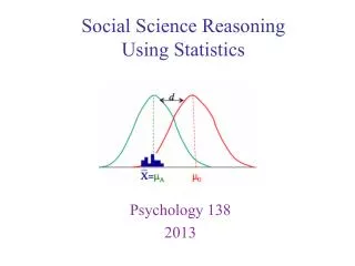
Social Science Reasoning Using Statistics Psychology 138 2018

Exam 2 is Wed. March 7th • Quiz 4 • Fri March 2nd • Covers z-scores, Normal distribution, and describing correlations Announcements

Transformations: z-scores • Normal Distribution • Using Unit Normal Table • Today’s lecture puts lots of stuff together: • Probability • Frequency distribution tables • Histograms • Z-scores Today Start the quincnux machine Outline

Number of heads HHH 3 HHT 2 HTH 2 HTT 1 THH 2 THT 1 TTH 1 TTT 0 Flipping a coin example

.4 .3 probability .2 .1 .125 .375 .375 .125 0 1 2 3 Number of heads Number of heads 3 2 2 1 2 1 1 0 Flipping a coin example

What’s the probability of flipping three heads in a row? .4 .3 probability .2 p = 0.125 .1 .125 .375 .375 .125 Think about the area under the curve as reflecting the proportion/probability of a particular outcome 0 1 2 3 Number of heads Flipping a coin example

What’s the probability of flipping at least two heads in three tosses? .4 .3 probability .2 p = 0.375 + 0.125 = 0.50 .1 .125 .375 .375 .125 0 1 2 3 Number of heads Flipping a coin example

What’s the probability of flipping all heads or all tails in three tosses? .4 .3 probability .2 p = 0.125 + 0.125 = 0.25 .1 .125 .375 .375 .125 0 1 2 3 Number of heads Flipping a coin example

Coin flipping results in The Binomial Distribution As you flip more coins, N = 20 Flipping a coin example

Coin flipping results in The Binomial Distribution As you flip more coins, the binomial distribution can be approximated by the Normal Distribution N = 65 Flipping a coin example

The Normal Distribution (Sometimes called the “Bell Curve”) • Many commonly occurring distributions in nature are approximately Normal Normal Distribution

Defined by density function (area under curve) for variable X given μ & σ2 • Symmetrical & unimodal; Mean = median = mode • Converting to standardized z-scores • The Normal Distribution (Sometimes called the “Bell Curve”) • Many commonly occurring distributions in nature are approximately Normal • Common approximate empirical distribution for deviations around a continually scaled variable (errors of measurement) • Mean = 0 • ±1 σ are inflection points of curve (change of direction) Normal Distribution

The Normal Distribution (Sometimes called the “Bell Curve”) • Many commonly occurring distributions in nature are approximately Normal • Common approximate empirical distribution for deviations around a continually scaled variable (errors of measurement) • Use calculus to find areas under curve (rather than frequency of a score) • We will use a table rather to find the probabilities rather than do the calculus. Galileo Gauss Check out the quincnux machine Normal Distribution

The Normal Distribution (Sometimes called the “Bell Curve”) • Important landmarks in the distribution (and the areas under the curve) • %(μ to 1σ) = 34.13 • p(μ < X < 1σ) + p(μ > X > -1σ) ≈ .68 • %(1σ to 2σ) = 13.59 • p(1σ < X < 2σ) + p(-1σ > X > -2σ) = 27%, cumulative = .95 • %(2σ to ∞) = 2.28 • p(X > 2σ) + p(X < -2σ) ≈ 5%, cumulative = 1.00 100% 95% 68% • We will use the unit normal table rather to find other probabilities 34.13 2.28 13.59 Normal Distribution

Lots of places to get the Unit Normal Table information • But be aware that there are many ways to organize the table, it is important to understand the table that you use • Unit normal table in your reading packet • And online: http://psychology.illinoisstate.edu/jccutti/psych138/resources copy/TABLES.HTMl - ztable • “Area Under Normal Curve” Excel tool (created by Dr. Joel Schneider) • Bell Curve iPhone app • Do a search on “Normal Table” in Google. Resources and tools

.4 .3 probability .2 • We will use the unit normal table rather to find other probabilities .1 .125 0 1 2 3 .875 Number of heads Unit Normal Table

Proportions beyondz-scores • Same p-values for+ and - z-scores • p-values = 0.50 to 0.0013 zp .1359+.0228 = .1587 For z = 1.00 , 15.87% beyond, p(z > 1.00) = 0.1587 1.01, 15.62% beyond, p(z > 1.00) = 0.1562 Note. : indicates skipped rows Unit Normal Table (in reading packet and online)

Proportions beyondz-scores • Same p-values for+ and - z-scores • p-values = 0.50 to 0.0013 For z = -1.00 , 15.87% beyond, p(z < -1.00) = 0.1587 100% - 15.87% = 84.13% = 0.8413 Note. : indicates skipped rows Unit Normal Table (in reading packet)

Proportions beyondz-scores • Same p-values for+ and - z-scores • p-values = 0.50 to 0.0013 For z = 2.00, 2.28% beyond, p(z > 2.00) = 0.0228 2.01, 2.22% beyond, p(z > 2.01) = 0.0222 As z increases, p decreases Note. : indicates skipped rows Unit Normal Table (in reading packet)

Proportions beyondz-scores • Same p-values for+ and - z-scores • p-values = 0.50 to 0.0013 For z = -2.00, 2.28% beyond, p(z < -2.00) = 0.0228 Note. : indicates skipped rows Unit Normal Table (in reading packet)

Proportions left of z-scores: cumulative • Requires table twice as long • p-values 0.0003 to 0.9997 50% + 34.13 = 84.13% to the left Cumulative % of population starting with the lowest value For z = +1, Unit Normal Tablecumulative version (in some other books)

Example 1 Suppose you got 630 on SAT. What % who take SAT get your score or better? 9.68% above this score • Population parameters of SAT: μ = 500, σ = 100, normally distributed From table: z(1.3) =.0968 • Solve for z-value of 630. • Find proportion of normal distribution above that value. Hint: I strongly suggest that you sketch the problem to check your answer against SAT examples

Example 2 Suppose you got 630 on SAT. What % who take SAT get your score or worse? 100% - 9.68% = 90.32% below score (percentile) • Population parameters of SAT: μ = 500, σ = 100, normally distributed From table: z(1.3) =.0968 • Solve for z-value of 630. • Find proportion of normal distribution below that value. SAT examples

Check the quincnux machine • In lab • Using the normal distribution • Questions? • Brandon Foltz: Understanding z-scores (~22 mins) • StatisticsFun (~4 mins) • Chris Thomas. How to use a z-table (~7 mins) • Dr. Grande. Z-scores in SPSS (~7 mins) Wrap up

Social Science Reasoning Using Statistics