Download
1 / 24
240 likes | 331 Views
Explore how statistical studies analyze relationships between two variables, cautionary notes on interpretations, the role of explanatory and response variables, and the significance of scatterplots in depicting quantitative relationships.

E N D
A medical study finds that short women are more likely to have heart attacks than women of average height, while tall women have the fewest heart attacks. An insurance group reports that heavier cars have fewer deaths per 100,000 vehicles than do lighter cars. These and many other statistical studies look at the relationship between two variables.
CAUTION: Statistical relationships are __________, not ______.They allow individual exceptions. For example, although smokers, on average, die younger than nonsmokers, some people live to 90 while smoking three packs a day. rules tendencies
To understand a statistical relationship between two variables, we measure both variables on the same individual. When analyzing a relationship between two variables, we must examine other variables as well. Name two variables that could affect the heart attack study above. weight, exersize, stress, heredity
Researchers need to eliminate the effect of these other variables. One of our main themes is that the relationship between two variables can be strongly influenced by other variables lurking in the background.
In chapter 3, we will focus on relationships between quantitative variables. Categorical variables will be examined in chapter 4. Quite often, you want to determine if one of the variables helps explain or even causes changes in the other.
An explanatory variablehelps explain or influences the changes in the response variable.
Explanatory variables are sometimes called independent variables and response variables are sometimes called dependent variables.
Example 1: Identify the explanatory and response variable in the following scenarios:
Alcohol has many effects on the body. One effect is a drop in body temperature. To study this effect, researchers give several different amount of alcohol to mice, then measure the change in each mouse’s body temperature in the 15 minutes after taking the alcohol.Explanatory: Response: amount of alcohol consumed change in body temperature
Jim wants to know how the mean 2005 SAT Math and Verbal scores in the 50 states are related to each other. He wants to determine if he can predict a state’s mean SAT Math score if he knows the mean SAT Verbal score.Explanatory:Response: mean SAT verbal score mean SAT math score
Note that in first scenario alcohol actually causes a change in body temperature. There is no cause-and-effect relationship between SAT Verbal and Math scores.
Caution: Calling one variable explanatory and the other responsive doesn’t necessarily mean that changes in one causechanges in the other.
The most effective way to display the relationship between two quantitative variables is with a scatterplot. To draw a scatterplot by hand: Plot the explanatory variable, if there is one, on the __________ ( __ ) axis of a scatterplot. If there is no explanatory-response distinction, either variable can go on the horizontal axis. Be sure to _______ and _______ both axes. The intervals on each axis must be uniform for that axis; and adopt a scale that uses the whole grid and allows the details to be easily seen. horizontal X label scale
Two variables are positively associatedwhen above average values tend to occur together on both variables.
Two variables are negatively associated when above average values on one variable tend to occur with below average values on the other.
When describing the overall pattern of a scatterplot you must address 3 key areas:direction (i.e.__________________________), form (i.e. ______________) andstrength (i.e ____________________________________) positive or negative association linear or curved how closely do the points follow the form
Also note unusual aspects such as clusters of points or points that lie far outside the pattern.Points that lie far away from all the others in the vertical direction are called ________Points hat lie far away from the others in the horizontal direction are ________________
NOTE: Always interpret scatterplots in the context of the problem.
Example 2: Interpret the scatterplot to the right:Direction:Form: Strength:Outliers: negative association slightly curved fairly strong Possible outlier at (20, 510)
To add a categorical variable to a scatterplot, use a different color or symbol for each category.
Scatterplots on the TI 83/84: 1. Put the data into two lists 2. STATPLOT (2ndfunc. of Y=) 3. Make sure all but the first are turned OFF 4. Turn plot1 ON and highlight the first graph and press ENTER 5. Xlistis the explanatory variable and Ylist is theresponse variable 6. Choose the “marker” you wish to use 7. Press GRAPH and ZOOM 9 for appropriate window
Example: How does the percent of adult birds in a colony from one year that return to nest the following year, affect the number of new birds that join the colony? Here are data for 13 colonies of sparrowhawks. Construct a scatterplot and describe what you see.% returning: 74 66 81 52 73 62 52 45 62 46 60 46 38# new birds: 5 6 8 11 12 15 16 17 18 18 19 20 20