Download
1 / 75
1.01k likes | 1.79k Views
The density matrix renormalization group. Adrian Feiguin. Some literature.

E N D
The density matrix renormalization group Adrian Feiguin
Some literature -S. R. White:. Density matrix formulation for quantum renormalization groups, Phys. Rev. Lett. 69, 2863 (1992).. Density-matrix algorithms for quantum renormalization groups, Phys. Rev. B 48, 10345 (1993). -U. Schollwöck. The density-matrix renormalization group, Rev. Mod. Phys. 77, 259 (2005). -Karen Hallberg . Density Matrix Renormalization: A Review of the Method and its Applications in Theoretical Methods for Strongly Correlated Electrons, CRM Series in Mathematical Physics, David Senechal, Andre-Marie Tremblay and Claude Bourbonnais (eds.), Springer, New York, 2003 . New Trends in Density Matrix Renormalization, Adv. Phys. 55, 477 (2006). -The “DMRG BOOK”: Density-Matrix Renormalization - A New Numerical Method in Physics: Lectures of a Seminar and Workshop held at the Max-Planck-Institut für Physik ... 18th, 1998 (Lecture Notes in Physics) by Ingo Peschel, Xiaoqun Wang, Matthias Kaulke and Karen Hallberg -R. Noack and S. Manmana . Diagonalization- and Numerical Renormalization-Group-Based Methods for Interacting Quantum Systems Proceedings of the "IX. Training Course in the Physics of Correlated Electron Systems and High-Tc Superconductors", Vietri sul Mare (Salerno, Italy, October 2004) AIP Conf. Proc. 789, 93-163 (2005) -A.E. Feiguin . The Density Matrix Renormalization Group and its time-dependent variants Vietri Lecture Notes. http://physics.uwyo.edu/~adrian/dmrg_lectures.pdf
Brief history and milestones • (1992) Steve White introduces the DMRG. • (1995-…) Dynamical DMRG. (Hallberg, Ramasesha et al, Kuhner and White, Jeckelmann) • (1995) Nishino introduces the transfer-matrix DMRG (TMRG) for classical systems. • (1996-97) Bursill, Wang and Xiang, Shibata, generalize the TMRG to quantum problems. • (1996) Xiang adapts DMRG to momentum space. • (2001) Shibata and Yoshioka study FQH systems. • (2004) Vidal introduces the TEBD. (time-evolving block decimation) • (2005) Verstraete and Cirac introduce an alternative algorithm for MPS’s and explain problem with DMRG and PBC. • (2006) White and AEF, and Daley, Schollwoeck et al generalize the ideas within a DMRG framework: adaptive tDMRG. … the DMRG has been used in a variety of fields and contexts, from classical systems to quantum chemistry, to nuclear physics…
Exact diagonalization “brute force” diagonalization of the Hamiltonian matrix. Schrödinger's Equation: H : Hamiltonian operator |x : eigenstate E : eigenvalue (ENERGY) H |x = E|x … anything you want to know… but… only small systems All we need to do is to pick a basis and write the Hamiltonian matrix in that basis
Exact diagonalization recipe Ingredients • Lattice (geometry) • Basis of states (representation) • Hamiltonian (model/interactions)
1D chain Ladder 2D Lattices
Boundary conditions Cylindrical Open Periodic
What degrees of freedom do we care about? valence band core electrons
Basis of statesOccupation number representation(1 orbital per site, spin ½) Spin up Empty Spin down Double occupied |2 |o |↓ |↑ States |x =|x1|x2|x3|x4....|xN Dimension = number of configurations = 4N N: number of lattice sites
Hamiltonian H=∑i,jHij Kinetic energy HK = -t (c†i↑cj↑+c†i↓cj↓+h.c.) HK |↑o = -t |o↑ On site interaction(diagonal) HU = U ni↑ni↓ HU |2 = U |2 U U→∞
Ising term (diagonal) HIsing= SizSjz HIsing |↑↓ = -J/4 |↑↓ HIsing |↑↑ = J/4 |↑↑ Spin flip HJ = J/2(Si-Sj++Si+Sj-) HJ |↑↓ = J/2 |↓↑
Hubbard model HHubbard= -t ∑<i,j>(c†i↑cj↑+c†i↓c j↓+h.c.)+U ∑ini↑ni↓ Heisenberg model HHeis= J ∑<i,j>SizSjz+ 1/2 (Si-Sj++Si+Sj-) t-J model Ht-J = -t ∑<i,j>Pt(c†i↑cj↑+c†i↓c j↓+h.c.)P+HHeis
Symmetries SH=HS Particle number conservation => Ntotal Spin conservations => Sztotal Spin reversal => |↑↓±|↓↑ Reflections D' = D / 2 Translations D' = D / N |yk = (1/M) ∑iaki Ti |f; aki =exp(ikxi)
Block diagonalization 0 0 0 0
1D chain ED Example: Heisenberg chain Model Hamiltonian: HHeis= J ∑<i,j>SizSjz+ 1/2 (Si-Sj++Si+Sj-) Geometry: Basis: |↑↓↑↓; |↓↑↓↑; |↑↑↓↓; |↓↑↑↓; |↓↓↑↑; |↑↓↓↑
Translations Applying translations: |1=1/(22){(1+ ei2k )|↑↓↑↓+ eik(1+ei2k)|↓↑↓↑} |2=1/2{|↑↑↓↓+eik|↓↑↑↓+ei2k|↓↓↑↑+ei3k|↑↓↓↑} With k=0,-/2, /2, |1=1/2{|↑↓↑↓+|↓↑↓↑} |2=1/2{|↑↑↓↓+|↓↑↑↓+|↓↓↑↑+|↑↓↓↑} k=0) k= -/2) |2=1/2{|↑↑↓↓+e-i/2|↓↑↑↓-|↓↓↑↑+ei/2 |↑↓↓↑} |2=1/2{|↑↑↓↓+ei/2|↓↑↑↓-|↓↓↑↑+e-i/2 |↑↓↓↑} k= /2) k= ) |1=1/2{|↑↓↑↓-|↓↑↓↑} |2=1/2{|↑↑↓↓-|↓↑↑↓+|↓↓↑↑-|↑↓↓↑}
Limitations : small lattices • Hubbard model: 20 sites at half filling, 10↑ and 10↓, D=20!(10!10!)x20!(10!10!) = 2.4e+10. After symmetries D'=1.1e+8 • t-J model (only |o, |↑and |↓ states): 32 sites with 4 holes, 14↑ and 14↓, D = 32!/(14!18!)x18!/(14!4!) = 1.4e+12; D'=5.6e9 • Heisenberg model (only |↑and |↓ states): 36 sites, 18↑ and 18↓, D = 36!/(18!18!)=9075135300; D' =D/(36x2x2x2x2)=1.5e6 states
Exact diag. is limited by system size… How can we overcome this problem? Po’ man’s solution: What about truncating the basis?
“Classical” analogyImage compression algorithms (e.g. Jpeg) We want to achieve “lossless compression” … or at least minimize the loss of information
Error = 1-∑' |ai|2 Cut here Idea 1: Truncated diagonalization , ∑ |ai|2 = 1 |gs =∑ ai|xi Usually, only a few important states possess most of the weight
Truncated diagonalization (continued) • We choose a small set of configurations that we know (from results in small systems) are important. E.g. |↑↓↑↓↑↓↑↓ • We apply the Hamiltonian H|x = |y, expanding the basis up to a dimension D. • We diagonalize and obtain the ground state: |gs =∑ai|xi • We order the weights |ai|2 in descending order • We truncate the basis keeping m states with larger weights • We go back to 2) until we reach convergence NOTICE: We are still working in the occupation number representation
Cut here Cut here |gs =∑ ai|xi , ∑ |ai|2 = 1 Error = 1-∑' |ai|2 Idea 2: Change of basis Can we rotate our basis to one where the weights are more concentrated, to minimize the error?
What does it mean “to truncate the basis” If we truncate This transformation is no longer unitary, does not preserve norm ->loss of information
The case of spins The two-site basis is given by the states |ss’ ={|↑↑;|↑↓;|↓↑; |↓↓} We can easily diagonalize the Hamiltonian by rotating with the matrix: That yields the eigenstates:
Let’s consider the 1d Heisenberg model For a single site , the operator matrices are: We also need to define the identity on a block of l sites
Building the Hamiltonian a la NRG 2 1 3 2 l-1 l This recursion will generate a 2lx2l Hamiltonian matrix that we can easily diagonalize
Another way to put it… l-1 l with
Adding a single site to the block Before truncating we build the new basis as: And the Hamiltonian for the new block as with
Idea 3: Density Matrix Renormalization Group S.R. White, Phys. Rev. Lett. 69, 2863(1992), Phys. Rev. B 48, 10345 (1993) |y = ∑ijyij|i| j Dim=2L Dimension of the block grows exponentially
Block decimation |y = ∑ijyij|i| j Dim=2N Dim=m constant
| = ∑ijij|i| j |' = ∑mjaj|| j The density matrix projection Universe system |i environment | j Solution: The optimal states are the eigenvectors of the reduced density matrix ii'=∑jiji'jTr= 1 with the m largest eigenvalues We need to find the transformation that minimizes the distance S=||'-||2
Understanding the density-matrix projection Universe system |i environment | j Region B Region A The reduced density matrix is defined as:
Properties of the density matrix • Hermitian -> eigenvalues are real • Eigenvalues are non-negative • The trace equals to unity-> TrrA=1 • Eigenvectors form an orthonormal basis.
The singular value decomposition (SVD) dimB Consider a matrix (we are choosing dimB < dimA for convenience) ij= dimA We can decompose it into the product of three matrices U,D,V: =UDV† • U is a (dimAxdimB) matrix with orthonormal columns-> UU†=1;U=U† • D is a (dimBxdimB) diagonal matrix with non-negative elements la • V is a (dimBxdimB) unitary matrix -> VV†=1 = U x x V D
This is also called the “Schmidt decomposition” of the state
The SVD and the density matrix In general: In the Schmidt basis, the reduced density matrix is • The singular values are the eigenvalues of the reduced d.m. squared wi=li2 • The two reduced density matrices share the spectrum • the singular vectors are the eigenvectors of the density matrix.
Optimizing the wave-function We want to minimize the distance between the two states S=||'-||2 where | is the actual ground state, and |’ is the variational approximation after rotating to a new basis and truncating |' = ∑mjaj|| j We reformulate the question as: Given a matrix ,what is the optimal matrix ’ with fixed rank r that minimizes the Frobenius distance between the two matrices. It turn out, this is a well known problem, called the “low rank matrix approximation”. If we order the eigenvalues of the density matrix in descending order w1,w2,…,wm,…,wr we obtain S=||'-||2 = Truncation error!
DMRG: The Algorithm How do we build the reduced basis of states? We grow our basis systematically, adding sites to our system at each step, and using the density matrix projection to truncate
1) We start from a small superblock with 4 sites/blocks, each with a dimension mi , small enough to be easily diagonalized m1 1 4 2 3 H1 The Algorithm • 2) We diagonalize the system and obtain the ground state |gs=∑y1234|a1|s2|s3|b4 • 3) We calculate the reduced density matrix rfor blocks 1-2 and 3-4. 4) We diagonalizer obtaining the eigenvectors and eigenvalues wi
m m2 m'1=mm2 • 5) We add a new site to blocks 1 and 4, expanding the basis for each block to m'1= mm2and m'4= m3 m • 7) We repeat starting from 2) replacing H1 by H'1andH4 by H'4 4 4 4 4 1 1 1 1 2 2 2 2 3 3 3 3 • 6) We rotate the Hamiltonian and operators to the new basis keeping the m states with larger eigenvalues (notice that we no longer are in the occupation number representation)
4 4 4 4 1 1 1 1 2 2 2 2 3 3 3 3 The finite size algorithm We add one site at a time, until we reach the desired system size
We sweep from right to left We sweep from left to right 1 1 1 4 4 4 4 4 4 4 4 4 4 4 4 2 3 1 1 4 1 1 1 1 1 1 1 1 2 2 2 2 2 2 2 2 3 3 2 3 3 3 3 3 3 3 2 3 3 2 2 3 The finite size algorithm …Until we converge
The discarded weight 1- ∑ma=1wa measures the accuracy of the truncation to m states
Observations • Sweeping is essential to achieve convergence • Run the finite-size DMRG and extrapolate to the thermodynamic limit. • For each system size, extrapolate the results with the number of states m, or fix the truncation error below certain tolerance.
Density Matrix Renormalization Group A variational method without a-priori assumptions about the physics. • Similar capabilities as exact diagonalization. • Can calculate properties of very large systems (1D and quasi-2D) with unprecedented accuracy. • Results are variational, but “quasi-exact”: Accuracy is finite, but under control.