Download
1 / 54
540 likes | 841 Views
CMPT 371. Data Communications and Networking Switching and throughput Multiplexing. Travels through a network. Data can travel along different paths from one station to another through the network. Station 2. Station 3. Station 1. Station 12. Station 14. Station 13. Station 7.

E N D
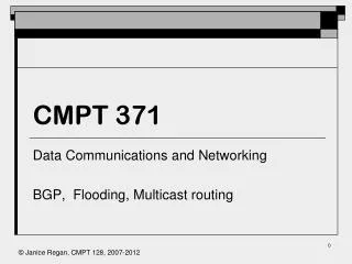
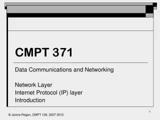
CMPT 371 Data Communications and Networking Switching and throughput Multiplexing
Travels through a network • Data can travel along different paths from one station to another through the network Station 2 Station 3 Station 1 Station 12 Station 14 Station 13 Station 7 Station 10 Station 6 Station 9 Station 6 Station 4 Station 5 Station 11
What is a hop Host 1 Host 1 First hop Host 1 is source Host 2 is receiver Host 2 Host 2 Second hop Host 2 is source Host 3 is receiver Host 3 Host 3
More Travel through a network • Does all data in a message take the same path? • What happens to data between each hop, what does each station do to the data passing through it ? Station 2 Station 3 Station 1 Station 12 Station 14 Station 13 Station 7 Station 10 Station 6 Station 9 Station 6 Station 4 Station 5 Station 11
Approached to network travel • We can take different approaches to managing data • Circuit switching: make a connection along a particular path and send all data in the message through that path • Packet switching: break the message into pieces and send each piece separately along its own path • Virtual circuit switching: break the message into pieces, Use software to simulate a connection in a packet switched network
Circuit Switching • Connection Oriented • A path or circuit, or series of hops through the network, from the sending station to the receiving station is established, used as dedicated link, then disconnected • The communications links used for the dedicated link are not available to other users for making other connections • Origin: analog telephone networks
Packet Switching • Packet Switching: Connectionless • The message is broken into packets. • Each packet travels through the network separately and can take a different path through the network • Each packet is transferred 1 hop at a time, The intermediate stations need only wait for the end of the packet not the end of the message • The communications links used to send the packet are not reserved for any particular connection and are available to all end systems
Virtual Circuit Switching • Used in packet switched networks • Uses software to simulate a connection • At any time any station can have multiple virtual circuit connections to the same or different destinations. • Virtual circuits allow retransmission of data packets that arrive with errors. Error/Flow control is associated with the virtual circuit
Packet Switching: virtual circuit • At the beginning of each data exchange between a source and a receiver, a single path or virtual circuit from the source to the receiver is established and all packets in the exchange follow this path. Since packets follow the same path they arrive in order • The virtual circuit is not dedicated. Each packet will be queued for transmission at each hop along with any other traffic traveling across that particular link. Thus, when the virtual circuit connection is not being used by the source and receiver in this exchange it may be used by other exchanges.
Circuit Switching • A path or circuit through the network is established. This path consists of a series of hops between nodes or switches, then a final hop to the receiver. • The switches have the intelligence to help determine a path through the network and allocate available resources • Once the circuit is established it is used as dedicated link • Data is transferred through that circuit, flow control is end to end (not hop by hop) • If data is in the form of a series of bursts, the time between bursts is not utilized. The utilization of the connection will be low if the data is a series of bursts • When the session is over the circuit is closed
Circuit Switching: Advantages • Provides a dedicated link • Efficient for continuous transmission • Do not have delay of waiting for packets to arrive before data can be forwarded along the next hop of the path • Easier to implement control for quality of service • Guaranteed bandwidth
Circuit Switching: Problems • Inefficient when data comes in bursts, during the time between bursts the connection is allocated but not being used • Overhead required to establish and break circuit • Connection must be reestablished if there is a problem with any switch along the established path • Cannot send at a rate higher than your allocated share of resources even if you are the only user
Packet switching • Each message sent is broken into small pieces called packets • Each packet is sent through the network separately • At each hop the packet must be forwarded to the next host along the path to the destination
Packet travel times • Packets can travel along different paths from one station to another • Different paths have different travel times • Packets that leave in order A-B-C may arrive in any order, because they travel along different paths with different travel times Station 10 Station 6 Station 9 Station 6 Station 4 Station 5 Station 11
Store and Forward node • A network node that • receives and stores incoming packets • checks incoming packets for bit level errors • Forwards the correct packets to the next store and forward node • Important: Think of each hop as a separate communication
Store and Forward node • Important: Think of each hop as a separate communication • Source sends packet • Receiver receives packet and queues it • If the queue is full the receiver drops the packet • Receiver checks the packet for correctness. • If a packet is not correct the receiver may drop the packet (best effort transmission) • Otherwise the receiver then passes packet on to another connection
Traffic Control on Networks Packet transmission time (transmission delay) After Figure 10.14 Stallings (2003)
Queuing delay • As the packet travels to each intermediate or final destination there are possible additional delays • Each time a packet arrives at a host or router or switch there is a possibility that it must enter a queue of packets waiting to be processed. • The time the packet resides in this queue, before the processing of the packet begins is the queuing delay
Queuing delay • When a packet arrives at a store and forward node, if the store an forward node is busy processing another packet it will be placed in a queue waiting for its turn. • Unlike other delays, different for different packets because the length of queue varies independent of the packet • Usually analyze queuing delays statistically
Processing delay • When a packet reaches a store and forward node • Its header must be read and analyzed • Its contents must be checked for bit level errors. • The time taken to do such checks is the processing delay.
Transmission delay • When a packet is sent the hardware used translates one bit at a time and inserts it onto the transmission medium. This operation takes time. • The time taken for all bits in the packet to be inserted into the transmission medium is the transmission delay
Propagation Delay • Each bit must travel from the source to the destination through the transmission medium • The time taken by each bit to travel from the source to the destination is the propagation delay
Packet loss • The length of the queue is finite, therefore when the system is busy it is possible for a packet to arrive and find there is no room in the queue: Such a packet is dropped • A packet may have bits corrupted in transmission. Such a packet will not pass the tests for bit level errors and will thus not reach the queue at all
Traffic Control on Networks Packet transmission time (transmission delay) After Figure 10.14 Stallings (2003)
Optimal Packet size • Consider the previous figure. The packet takes a 3 hop path through the network • Message could sent as a single packet: message switching • Message could be broken into smaller packets: packet switching • How do we determine the optimal size for a packet/message
Single message • Consider the previous figure. The packet takes a 3 hop path through the network • Message is sent as a single packet: message switching • The amount of added overhead due to packet headers is minimal since only one packet header is needed • the intermediate nodes must wait until the entire packet has arrived before the packet can be FCS checked and queued for transmission across the next hop. (longer wait)
Packets • Consider the previous figure. The packet takes a 3 hop path through the network • When the message is broken into smaller packets (packet switching) • The amount of added overhead due to packet headers increases as the size of the packet decreases • The delay, waiting for each packet to arrive, at each intermediate node is reduced as the length of the packets are reduced • The amount of data to be retransmitted if a packet is lost is reduced
Effect of packet size Stallings 2003: Figure 10.14
Optimal Packet size • First consider the delay for the single packet case where Tp,transmission time of the packet Thtransmission time of the header Tproppropagation time per transmission Ntrans# of time the signal is transmitted
Optimal Packet size • For the two packet case • For the five packet case • Therefore we can generalize the relation to • For #hops equal to Ntrans -1 (alternate definition)
Packet size considerations • Delay is introduced by requiring packet, or section of message, to arrive at an intermediate station before the message is forwarded is smaller than for message switching • Shorter packets are less likely to contain errors and require retransmission than long messages • Packet headers add additional overhead that increases as the size of the packet decreases • Waits for next link will be minimized if smaller packets of data are being transmitted as single units • Required retransmissions are shorter, and add less additional load to the system
Packet Switching: • No call setup or call termination required. • Each packet, referred to as a datagram, is sent individually, and is routed through the network individually • Packets with the same source and destination may take different paths through the network and thus may arrive at the receiver out of order • Flexible reaction to congestion and failure • Robust delivery of packets, less loss of information in lost packet than in broken virtual connection when a node fails
Multiplexing • When multiple signals are carried through a single transmission medium at the same time, the signals are multiplexed • Multiplexing allows the efficient use of wider band transmission media. Such media can carry multiple narrower band signals. • Long haul links are frequently examples of high capacity channels • The multiple signals must be combined or multiplexed in such a way that the individual signals can be easily extracted from the composite signal (demultiplexed) on reception
Methods of Multiplexing • Frequency Division Multiplexing • Time Division Multiplexing • Synchronous • Statistical • Code Division Multiplexing (spread spectrum) Diagram Stallings 2003:Figure 8.1
FDM and TDM Stallings 2003:Figure 8.2
Frequency Division Multiplexing • When the transmission media has a bandwidth many times larger than the bandwidth of the signal to be transmitted, it makes sense to transmit more than one signal at a time through the medium. • Each of the signals to be transmitted are modulated to a different carrier frequency. • The different carrier frequencies are separated by at least the bandwidth of the individual signals to be transmitted • The frequency bandwidth is shared by the signals being simultaneously transmitted
Frequency division multiplexing Bandwidth of Medium is fmax-fmin f7 f1 f2 f3 f4 f5 f6 f8 fmax fmin f(i+1}=fi + bandwidth of signal Bandwidth of each signal
FDM • Examples of FDM include multiplexing of voice signals over telephone lines, and multiplexing of cable channels into the allocated cable frequency band • FDM can be done in stages. M signals can be multiplexed into a particular frequency band. Groups of M signal can then be combined and multiplexed into a larger frequency band
FDM multiplexing system Stallings 2003:Figure 8.3
FDM and voice signals: 1 • A typical voice signal has an effective spectrum of 300 to 3400 Hz, When multiplexing signals the signals must be adequately separated, so allow 4KHz bandwidth for each voice signal • A voice signal can be modulated so that the spectrum of the modulated signal has a center frequency at the frequency of the modulation carrier fc, • If the carrier has a bandwidth between f1 Hz and f2 Hz then fc would be chosen to be f1+4KHz
Cable and ADSL • ADSL uses the fixed telephone system. • Each user has a dedicated connection to the end office • User must be close enough to the end office • Each of these connections use twisted pair • Capacity of twisted pair less than capacity of cable • Uses FDM • Cable shares a higher capacity coaxial cable between multiple users. • Available capacity may be higher or lower than ADSL • Can intercept packets of other users on the same cable link • Uses TDM
ADSL access to Internet Telecom’s Internet Access LOCAL PHONE OFFICE TELEPHONE SWITCH & DSLAC: Digital Subscriber Line Access Multiplexer
Cable access to Internet Cable Providers Internet Access
ADSL • Asymmetric Digital Subscriber Line, to 8Mbps downstream and 1Mbps upstream. (Typically 512 kbps and 64 kbps) • Provides high speed access over twisted pair telephone wires. Up to 256 4MHz channels available • Normal telephone connection filtered to 4KHz bandwidth at end office (switching station) • For ADSL filter is removed making entire capacity of the twisted pair (category 3) available to the user. The capacity and attainable speed depend on the distance from the end office (length of connection). • Typical user needs more downstream capacity than upstream capacity for internet applications • Uses FDM and/or discrete multitone (DMT)
Wavelength Division Multiplexing • Used with optical fibre • Light passing through the fiber consists of many colours or wavelengths (frequencies) • Each wavelength carries a signal • The fibre can carry many signals at the same time, as signals with different wavelengths • As many as 160 channels at 10 Gbps • Used for cable (between central offices)
TDM (Time Division) • The data are organized in frames • Each frame contains a cycle of time slots • A sequence of slots dedicated to one source is a channel • Data from different sources is inserted into slots or channels in some sequence • Synchronous TDM slots are filled from a predetermined sequence of sources. If there is no data to transmit an ‘idle’ signal is sent (circuit switching) • Statistical TDM fills slots as data is available. There is not preset sequence. Therefore, data must be associated with the source by address. No empty or ‘idle’ slots are sent if any source has data ready to transmit. Idle is sent only if all channels have no data to transmit (packet switching)
Synchronous TDM Cycle of time slots Channel (1 or more slots) Stallings 2003:Figure 8.6
Statistical TDM • Time slots are not preallocated to particular sources, they are allocated on demand. • There are M sources, N available channels .: M>=N • Rather than transmitting an idle signal when no data is available from a source i, data from source j can be transmitted. • The data rate of the transmission line can be smaller than the sum of the data rates for all sources being serviced • At peak times the data rate of received data from the sources may exceed the data rate of the transmission media. In these cases excess data must be buffered in the multiplexer for later transmission
Statistical TDM • Statistical TDM is most useful is systems where sources do not broadcast continuously. • If each source broadcasts 80% of the time. Statistical TDM can handle 20% more channels than asynchronous TDM • There are overhead costs associated with this gain in efficiency. • Sources are not transmitted in a predetermined order, so there is not a direct way to know which source is being transmitted in a given channel. Thus, each channel must contain an address that indicates the source