Download
1 / 80
800 likes | 821 Views
Learn the foundations of causality interpretation, different causal effects, and ways to confirm causality. Grasp Granger causality, conditional effects, multicollinearity, orthogonality, and hidden causes. Discover the importance of storytelling in data analysis for more accurate conclusions.

E N D
Causality TRIBE statistics course Split, spring break 2016
Goal Understand that causality bases on interpretation, not data Know different types of causal effects Ways to confirm causality
Motivation Predictability Dimensions • understand (a goal per se) • control (know what to influence) • trade off (efficient intervention) • Even stochastic settings can be assessed by means of simulations
Analytical problem • Relations invertible • y = f(x) <=> x = f-1(y), but not always unique • Correlation (X, Y) = correlation (Y, X)
Granger causality Determines whether one time series is useful to forecast the other Everybody knows it, few (at least econometricians) use it Usually challenged when applied
Granger causality in EViews Quick Group Statistics Granger • Selection of lags usually involves a tradeoff bias versus power • (The example does not make sense since we have no time series)
Timing The 'normal' case • Early events cause later ones • Simultaneous reaction also occursNewton's third law of motion:Action leads to reaction • An effect cannot precede its cause
Counterexample Rational expectations Social sciences • Inflation bias • Measures that take effect in the future and induce adjustments today • Pricing of financial assets (in principle, only the future is relevant) Expectations can drive action but depends on • Availability of information • Time-consistent behavior • Rational decision making
Stability Predictions • No risk safe • Stochastic realizations likelihood function • No distributional information ? Regime switches as a possibility of distribution for the distribution • Breaks • Transition matrix, which may also evolve over time • Rarely hybrid functional forms (too many parameters)
Global effects Global effect means that a change in X influences all realizations of Y Standard • Indifference => no effect of X on Y • Linear relations => uniform effect of input changes • Marginal effects vary => functional forms of the relation The form of the relation usually • exhibits few parameters (for example the logarithm) • remains stable (also reduces parameters) • stems from the story behind
Conditional effects Causal effects do not necessarily apply equally for all variables X The ponytail example • Suppose a man likes women and even more so those with ponytails • A woman can likely change her attractiveness (for him) via haircut • For another man, the haircut route is also open but less promising Conditional effects are usually captured by dummies
Multicollinearity High (linear) correlation among predicting variables (X)(applies for other relations than linear ones as well) Quantitative blindness • Similar (even identical) variables are equally likely to cause an effect • No quantitative way to distinguish the individual effects • Story behind the theory decisive As a remedy, drop correlated variables (loss in explanatory power not dramatic since there is redundancy exactly due to the correlation), use partial regressions or principal component analysis
Orthogonality Moving in parallel to one axis, no change on the other occurs Errors should be orthogonal to X (otherwise, X could explain more)
Principal component analysis (PCA) Works like linear OLS but rotates the direction of the axes Components are orthogonal but combinations of all dimensions (Pictures do refer to similar but not identical data)
Instrumental variables • Problem Y may influence X (reverse causality) • Situation Experiments are not possible • Solution Instrument that is correlated with X but not with ε Result: consistent estimators for the effect of X on Y
Hidden causes The observed variable may not capture the real driving force • The data collecting situation may differ from real life(only a game, political correctness, etc.)=> Bias especially at budgets and preferences • No problem as long as the relation from hidden to observed is stable(at least with respect to quantitative aspects as predictions)=> Dangerous if one wants to apply the insights in a different field • Yet unknown forces(rare, but a standard scientific alternative)=> Sensibility for different explanation approaches valuable
Story before data Comovements (also in opposite directions and not necessarily linear) suggest causality in one or both directions but do not imply it Experiments may solve the problem of causality controlling for the • interaction of external factors with the result • interaction of external factors with the explanation • unbiased data collection With respect to causality, the story is more important than the data
To do list Construct a story Remain open for alternative explanations in terms of the story Exclude conceivably causal unmeasured variables in experiments Look for instrumental variables if the error varies with the outcome In case of causality, assess the size and efficiency of the effect
Conclusion • Strong (large and invariable) effects support the idea of causality • Causal effects can affect subsamples differently • Principal component analysis indicates the minimum number of relevant dimensions for the sample variation and their importance • Instrumental variables can disentangle effects of reverse causality • Causality generally unsolved in theory=> Decide on the basis of the story, not of the data
Correlation TRIBE statistics course Split, spring break 2016
Goal Know the standard correlation measures Link correlation, causality, and independence See the link from correlation to explanatory content in regressions
Nonlinear correlation Connection, but not linear – measurable, but no easy standard
Pearson's ρ For linear correlations • ρfor the population • equivalent formulation in z-scores (standardized X and Y) • sometimes called r in a sample Rule of thumb: weak up to an absolute value of 0.3, strong from 0.7 on
Linear correlation (values of Pearson's ρ) The slope is NOT decisive for the strength of the correlation
Spearman's ρ For rank data (difficulties with ties Kendall's tau) • definition • d = difference in statistical rank of the corresponding variables • r is an approximation to the exact correlation coefficient Σxy/√Σx2Σy2
Pearson versus Spearman Can you imagine a situation where Pearson's ρ is higher?
Correlation in EViews Quick Group Statistics Correlations
t-statistic a and p-value for correlation in EViews Group View Covariance Analysis
More than 2 dimensions Possible for one dimension with respect to several ones Pearson's ρ between one variable and its linear predictor by the others Rarely used since it implies a regression (with intercept), and if one does already that, the regression output offers more information
Independence Independence => no correlation, but not necessarily the other way If two variables are jointly normally distributed (but not if they are only individually normal), no correlation also implies independence If Y is a (non-constant) function of X, X and Y are always dependent • Correlation is not sufficient for causality • Independence is not sufficient to exclude correlation Reason: Measured outcome due to chance or third factors
Transformation Asymmetric transformations • not the same operation on X and Y (usually only on one of the two) • Goal = construct a linear relation • Basis for linear OLS regressions Symmetric transformations • if monotonic, like taking the natural logarithm of both X and Y • do not change the correlation • get chosen mainly for the sake of visualization (different stretch) Caveat: Transformation affects the gap (= error in a regression), too
First choice transformations Often recommended transformations: • Logarithmic transformation for absolute values, usually y = ln(x) • Square-root transformation for absolute frequencies • Arcsin transformation for relative frequencies (in percent)
Subsets Eye inspection may hint at different correlation across subsets of X/Y • Scatter plot in EViews: Quick Graph (select series) Scatter
Link to OLS • Pearson's ρ = √R2 in a univariate linear OLS regression
Spuriousness Spurious relation • Correlation can be due to random variation • In most (and the worst) cases, true driver of correlation = a 3rd factor • Story becomes crucial (again) Types • Relation • Correlation: for ratios by the same (even if independent) variable • Regression: 'In short, it arises when we have several non-stationary time-series variables, which are not cointegrated, and we regress one of these variables on the others.' (example by Dave Giles)
To do list Apply eye inspection to your data (and common sense) Infer dependence from correlation, but not automatically causality Also apply ranking correlation to metric data (non-linear relation) Find a simple transformation that leads to a normal distribution Try the correlation of transformed variables (for new ideas)
Conclusion • Correlation is a measure of linear co-movement of two variables • Correlation due to chance, causality, or third factors (not exclusive) • Correlation ≠ 0 does neither exclude nor imply causality • Correlation ≠ 0 does not occur under independence • Correlation2 = explanatory content in the corresponding regression
Linear OLS regression TRIBE statistics course Split, spring break 2016
Goal Understand the optimization criterion for OLS regressions Implementation in EViews including extensions(dummies, interaction terms, lags) Interpretation of linear regressions
Motivation Usually, one looks for a (causal) relationship rather than independence • Model for the relation, Y = f(X) • Dependent variable(s) explained (partially) by independent ones • Dependence among X also possible Researchers would like to tell a story that • explains the data • people understand • predicts well (also situations previously not experienced)
Why linear? Easy • Computation (important in the early days) • Expansion (Y and X variables, effect types, lags) • Interpretation Constant marginal effects • Few parameters (less data needed and/or less uncertainty) • Extrapolation (to zero, full support, even for questionable situations) • Predictions for any input combination X (also negative values)
Why OLS? Goal = small distance to the data (points) • 'Better' (here: smaller) along 1 dimension usually easy to define • With several dimensions, however, tradeoffs arise => preferences • OLS focuses on the Y dimension and does not entangle dimensions Least squares • Mathematically and computationally easy • Unique (unlike 'least absolute distance' for example) • Concept adoptable for distances to other than straight lines
Linear regression in EViews Quick Estimate equation… enter equation, here 'weight c height'
Resulting model Intercept, marginal effects, (assumedly) normal error term Usually aiming from the beginning at a rejection of the H0(or at least of the H0 referring to a zero slope) Goes through the average of X and Y, heavily affected by outliers
Explanatory content (R2) How much of the H0 'deviation' disappears with the OLS line R2 = 1 - (Sum of squared residuals)/(Sum of squared deviations) Compare the 'best' straight line with H0 (usually the flat straight line)
R2 Explanatory content increases inevitably with additional X variables (unless they are perfectly collinear with a previous explanatory variable) => adjusted R2: compensates roughly for the additional dimension of X Large Y categories can lead to artificial and potentially large residuals even with a perfect model Alternative: total least squares: hardly ever used because it mixes up the two (or more) dimensions => Principal Component Analysis (PCA)