Download
1 / 42
420 likes | 642 Views
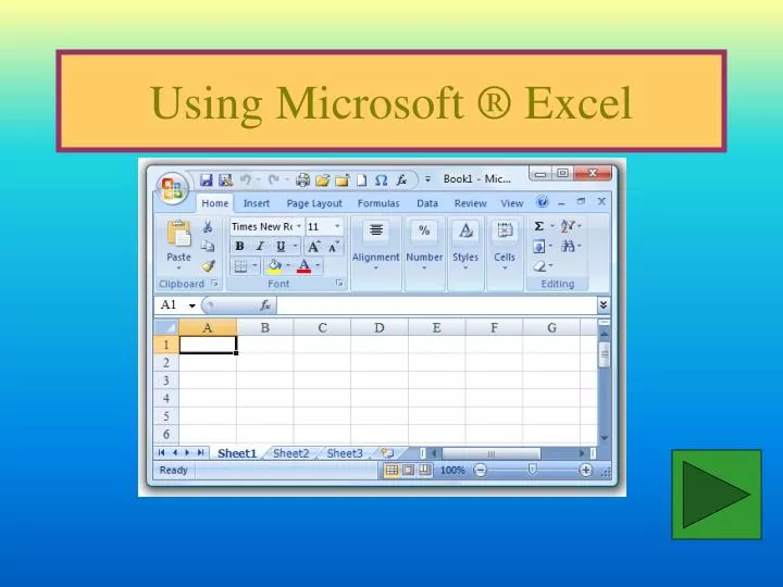
Using Microsoft ® Excel. Formulas and Functions. Start Microsoft ® Excel . Type data into cells as shown. Calculating PERCENT. Select cell D1 . Type the formula: =B2/C2*100 . Press Enter . Copying the Formula I.

E N D
Formulas and Functions • Start Microsoft ® Excel. • Type data into cells as shown.
Calculating PERCENT • Select cell D1. • Type the formula: =B2/C2*100. • Press Enter.
Copying the Formula I • Click and drag the heavy dot in the lower right hand corner of cell D2. • Drag downwards to fill cells D3 to D10.
Copying the Formula II • Release the mouse button to calculate the Percent.
Inserting a Function I • Click on cell B12. • Click on the Formulas tab. • Select Insert Function. • A dialog box will be displayed.
Inserting a Function II • Scroll down and select the SUM function. • Click OK.
Inserting a Function III • Type the range B2:B10 beside Number1. • Click OK.
Inserting a Function IV • The sum of the marks is calculated and displayed in cell B12.
Copying the Function • Drag the lower right hand corner of cell B12 to copy the function to cell C12.
Calculating the Midterm Mark • Click on cell D12. • Type the formula: =B12/C12*100. • Press Enter. • Note the midterm mark in cell D12.
Cell References I • In the previous example, you copied formulas, such as the one in cell B12 to cell C12. • Note that the cell reference B2:B10 was changed to C2:C10 for the formula in C12. • This is called relative cell referencing.
Cell References II • Sometimes you will want to keep a cell reference the same as you copy. An example is an interest rate in a compound interest table. • In this example, the interest rate is in cell B1. To keep the reference absolute, use a $ sign before both the row and column references when you enter the formula =B5*(1+$B$1/100) in cell B6. As you copy this formula down column B, the reference to $B$1 will remain constant.
Using the Fill Feature I • You can also use the Fill feature under the Edit menu to copy functions and formulas. • To see how this works, start a new sheet and enter the data shown into columns E and F.
Using the Fill Feature II • Select cells E2 to E15. • Select the Fill button on the Home/Editing menu. • Select Series… .
Using the Fill Feature III • Select options as desired. • Click OK.
Using the Fill Feature IV • The column is automatically filled with the numbers from 1 to 15.
Using the Fill Feature V • Enter the formula =1.8*E2+32 in cell F2. • Click and drag to highlight cells F2 to F16.
Using the Fill Feature VI • Select the Fill button on the Home/Editing menu. • Select Series…. • Select AutoFill. • Click OK.
Using the Fill Feature VII • Note that the formula has been copied through cell F16.
Charting I • A spreadsheet can be used to draw charts and graphs. • Start a new sheet and enter the data shown.
Charting II • Select cells A1 to A7. • Hold the Ctrl key and select cells G1 to G7.
Charting III • Click on he Insert tab. • Select Column. • Select the first 2D Column option.
Charting IV • A column chart will be displayed. • You can use other options to label axes, select gridlines, etc.
Sorting I • A spreadsheet can be used to sort data. • Click and drag to highlight the data.
Sorting II • Select the Data tab. • Click on Sort.
Sorting III • Select Points as the first sort column, and adjust other options. • Add a level to sort by Wins. • Then, sort by Losses. • Click OK.
Sorting IV • A three-stage sort has been performed on the data.
Search I • A spreadsheet can find or replace data using the Find & Select feature in the Editing group.
Search II • Suppose you want to replace all of the 5s in the previous spreadsheet with 6s. • Select all of the data cells. Then, select Replace…. • In the Find what box, type 5. • In the Replace with box, type 6. • Choose Replace All.
Search III • Note that all of the 5s have been replaced with 6s.
Filtered Search I • A spreadsheet can be used to filter data. For example, suppose that we want to select only those teams with less than 16 points. • Select the data from cell A1 to cell G7. • Click on the Data tab. • Select Filter.
Filtered Search II • Pull down the menu in the POINTS column. • Select Number Filters, then Less than… . • Add a 16 as shown, and click OK.
Filtered Search III • Note that the data have been filtered according to the desired parameter.
Adding and Referencing Worksheets I • You can have several worksheets within a file. Data on one sheet can contain a reference to data on another. • Sheets are selected using the tabs at the bottom of the screen.
Adding and Referencing Worksheets II • Hold down the Ctrl key while you click and drag to highlight the TEAM, GF, and GA columns. • From the Clipboard group, select Copy.
Adding and Referencing Worksheets III • Click on Sheet2. • Pull down the Paste menu and select Paste Special. • Click on Paste Link.
Adding and Referencing Worksheets IV • Click on cell B2. • Notice that it contains a reference to cell E2 on Sheet1. • If you change cell E2 on Sheet1, then cell B2 on Sheet2 will also change. • If you change cell B2 on Sheet2, cell E2 on Sheet1 will not change.
Adding and Referencing Worksheets V • You can manipulate the data on Sheet2 without affecting Sheet1. To see how this works, select Sheet2. • Click and drag to select the data from cell A1 to cell C7. • Pull down the Data menu and select Sort. Set the sort parameters as shown at the right. Then, click OK.
Adding and Referencing Worksheets VI • Notice that Sheet2 is now sorted. However….
Adding and Referencing Worksheets VII • ...Sheet1 is not.
The End • This concludes the tutorial presentation on using Microsoft ® Excel. • For more information visit: www.mcgrawhill.ca/links/MDM12