Download
1 / 32
320 likes | 364 Views
Learn how to compare population proportions, conduct hypothesis testing, estimate differences, and calculate confidence intervals using different formulas and statistical methods.

E N D
Independent Samples: Comparing Proportions Lecture 41 Section 11.5 Mon, Nov 21, 2005
Comparing Proportions • We now wish to compare proportions between two populations. • Normally, we would be measuring proportions for the same attribute. • For example, we could measure the proportion of NC residents living below the poverty level and the proportion of VA residents living below the poverty level.
Examples • The “gender gap” – the proportion of men who vote Republican vs. the proportion of women who vote Republican. • The proportion of teenagers who smoked marijuana in 1995 vs. the proportion of teenagers who smoked marijuana in 2000.
Examples • The proportion of patients who recovered, given treatment A vs. the proportion of patients who recovered, given treatment B. • Treatment A could be a placebo.
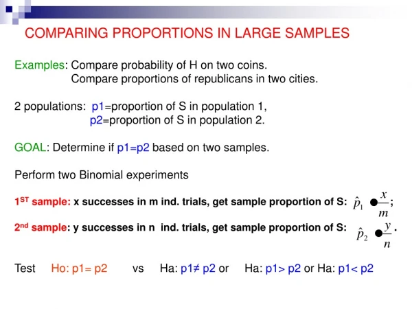
Comparing proportions • To estimate the difference between population proportions p1 and p2, we need the sample proportions p1^ and p2^. • The difference p1^ – p2^ is an estimator of the difference p1 – p2.
Hypothesis Testing • See Example 11.8, p. 721 – Perceptions of the U.S.: Canadian versus French. • p1 = proportion of Canadians who feel positive about the U.S.. • p2 = proportion of French who feel positive about the U.S..
The hypotheses. • H0: p1 – p2 = 0 (i.e., p1 = p2) • H1: p1 – p2 > 0 (i.e., p1 > p2) • The significance level is = 0.05. • What is that test statistic? • That depends on the sampling distribution of p1^ – p2^.
The Sampling Distribution of p1^ – p2^ • If the sample sizes are large enough, then p1^ is N(p1, 1), where • Similarly, p2^ is N(p2, 2), where
The Sampling Distribution of p1^ – p2^ • Therefore, where
The Sampling Distribution of p1^ – p2^ • The sample sizes will be large enough if • n1p1 5, and n1(1 – p1) 5, and • n2p2 5, and n2(1 – p2) 5.
The Test Statistic • Therefore, the test statistic would be if we knew the values of p1 and p2. • We could estimate them with p1^ and p2^. • But there is a better way…
Pooled Estimate of p • In hypothesis testing for the difference between proportions, typically the null hypothesis is H0: p1 = p2 • Under that assumption, p1^ and p2^ are both estimators of a common value (call it p).
Pooled Estimate of p • Rather than use either p1^ or p2^ alone to estimate p, we will use a “pooled” estimate. • That is the proportion that we would get if we pooled the two samples together.
The Standard Deviation of p1^ – p2^ • This leads to a better estimator of the standard deviation of p1^ – p2^.
Caution • If the null hypothesis does not say H0: p1 = p2 then we should not use the pooled estimate p^, but should use the unpooled estimate
The Test Statistic • So the test statistic is
The Value of the Test Statistic • Compute p^: • Now compute z:
The p-value, etc. • Compute the p-value: P(Z > 7.253) = 2.059 10-13. • Reject H0. • The data indicate that a greater proportion of Canadians than French have a positive feeling about the U.S.
Exercise 11.34 • Sample #1: 361 “Wallace” cars reveal that 270 have the sticker. • Sample #2: 178 “Humphrey” cars reveal that 154 have the sticker. • Do these data indicate that p1 p2?
Example • State the hypotheses. • H0: p1 = p2 • H1: p1p2 • State the level of significance. • = 0.05.
Example • Write the test statistic.
Example • Compute p1^, p2^, and p^.
Example • Now we can compute z.
Example • Compute the p-value. • p-value = 2 normalcdf(-E99, -3.126) = 2(0.0008861) = 0.001772. • The decision is to reject H0. • State the conclusion. • The data indicate that the proportion of Wallace cars that have the sticker is different from the proportion of Humphrey cars that have the sticker.
TI-83 – Testing Hypotheses Concerning p1^ – p2^ • Press STAT > TESTS > 2-PropZTest... • Enter • x1, n1 • x2, n2 • Choose the correct alternative hypothesis. • Select Calculate and press ENTER.
TI-83 – Testing Hypotheses Concerning p1^ – p2^ • In the window the following appear. • The title. • The alternative hypothesis. • The value of the test statistic z. • The p-value. • p1^. • p2^. • The pooled estimate p^. • n1. • n2.
Example • Work Exercise 11.34 using the TI-83.
Confidence Intervals for p1^ – p2^ • The formula for a confidence interval for p1^ – p2^ is • Caution: Note that we do not use the pooled estimate for p^.
TI-83 – Confidence Intervals for p1^ – p2^ • Press STAT > TESTS > 2-PropZInt… • Enter • x1, n1 • x2, n2 • The confidence level. • Select Calculate and press ENTER.
TI-83 – Confidence Intervals for p1^ – p2^ • In the window the following appear. • The title. • The confidence interval. • p1^. • p2^. • n1. • n2.
Example • Find a 95% confidence interval using the data in Exercise 11.34.