Download

1 / 66
660 likes | 691 Views
Explore optimal buffer management and scheduling strategies, from FIFO queuing to weighted round-robin and Deficit Round-Robin algorithms. Understand fairness, performance bounds, and trade-offs in scheduling disciplines.

E N D
Buffer Scheduling • Who tosend next? • What happens when buffer is full? • Who to discard?
Requirements of scheduling • An ideal scheduling discipline • is easy to implement • is fair and protective • provides performance bounds • Each scheduling discipline makes a different trade-off among these requirements
Ease of implementation • Scheduling discipline has to make a decision once every few microseconds! • Should be implementable in a few instructions or hardware • for hardware: critical constraint is VLSI space • Complexity of enqueue + dequeue processes • Work per packet should scale less than linearly with number of active connections
Fairness • Intuitively • each connection should get no more than its demand • the excess, if any, is equally shared • But it also provides protection • traffic hogs cannot overrun others • automatically isolates heavy users
Max-min Fairness: Single Buffer • Allocate bandwidth equally among all users • If anyone doesn’t need its share, redistribute • maximize the minimum bandwidth provided to any flow not receiving its request • To increase the smallest need to take from larger. • Consider fluid example. • Ex: Compute the max-min fair allocation for a set of four sources with demands 2, 2.6, 4, 5 when the resource has a capacity of 10. • s1= 2; • s2= 2.6; • s3 = s4= 2.7 • More complicated in a network.
FCFS / FIFO Queuing • Simplest Algorithm, widely used. • Scheduling is done using first-in first-out (FIFO) discipline • All flows are fed into the same queue
FIFO Queuing (cont’d) • First-In First-Out (FIFO) queuing • First Arrival, First Transmission • Completely dependent on arrival time • No notion of priority or allocated buffers • No space in queue packet discarded • Flows can interfere with each other; No isolation; malicious monopolization; • Various hacks for priority, random drops,...
Priority Queuing • A priority index is assigned to each packet upon arrival • Packets transmitted in ascending order of priority index. • Priority 0 through n-1 • Priority 0 is always serviced first • Priority i is serviced only if 0 through i-1 are empty • Highest priority has the • lowest delay, • highest throughput, • lowest loss • Lower priority classes may be starved by higher priority • Preemptive and non-preemptive versions.
Packet discard when full High-priority packets Transmission link Low-priority packets When high-priority queue empty Packet discard when full Priority Queuing
Flow 1 Transmission link Flow 2 Round robin Flow 3 Round Robin: Architecture • Round Robin: scan class queues serving one from each class that has a non-empty queue Called also: Cyclic Polling with limited-1 service Hardware requirement: Jump to next non-empty queue
Round Robin Scheduling • Round Robin: scan class queues serving one from each class that has a non-empty queue
Round Robin (cont’d) • Characteristics: • Classify incoming traffic into flows (source-destination pairs) • Round-robin among flows • Problems: • Ignores packet length (GPS, Fair queuing) • Inflexible allocation of weights (WRR,WFQ) • Benefits: • protection against heavy users (why?)
Weighted Round-Robin • Weighted round-robin • Different weight wi(per flow) • Flow j can sends wjpackets in a period. • Period of length wj • Disadvantage • Variable packet size. • Fair only over time scales longer than a period time. • If a connection has a small weight, or the number of connections is large, this may lead to long periods of unfairness. Called also: Cyclic Polling with limited Wj service
DRR (Deficit RR) algorithm • Like RR (over bits), variable packet size • Choose a quantum of bits to serve from each connection in order. • For each HoL (Head of Line) packet, • credit := credit + quantum • if the packet size is ≤ credit; send and save excess, • otherwise save entire credit. • If no packet to send, reset counter (to remain fair) • If some packet sent: counter = min{ excess, quantum } • Each connection has a deficit counter (to store credits) with initial value zero. • Easier implementation than other fair policies • WFQ To prevent Volume attack by Flow that sends many small packets
Deficit Round-Robin • DRR can handle variable packet size Quantum size : 1000 byte • 1st Round • A’s count : 1000 • B’s count : 200 (served twice) • C’s count : 1000 • 2nd Round • A’s count : 500 (served) • B’s count : 0 • C’s count : 800 (served) 2000 1000 0 1500 A 300 B 500 1200 C Head of Queue Second Round First Round
DRR: performance • Handles variable length packets fairly • Backlogged sources share bandwidth equally • Preferably, packet size < Quantum • Simple to implement • Similar to round robin
Generalized Process Sharing (GPS) • The methodology: • Assume we can send infinitesimal packets • single bit • Perform round robin. • At the bit level • Idealized policy to split bandwidth • GPS is not implementable • Used mainly to evaluate and compare real approaches. • Has weights that give relative frequencies.
GPS: Example 1 (PS) 60 50 30 Packets of size 10, 20 & 30 arrive at time 0
GPS: Example 2 (PS) 40 45 15 5 30 Packets: time 0 size 15 time 5 size 20 time 15 size 10
GPS: Example 3 (PS) 15 5 30 60 45 Packets: time 0 size 15 time 5 size 20 time 15 size 10 time 18 size 15
GPS : Adding weights • Flow j has weight wj • The output rate of flow j, Rj(t) obeys: • For the un-weighted case (wj=1):
Fairness using GPS • Non-backlogged connections (received what they asked for). • Backlogged connections: share the remaining bandwidth in proportion to the assigned weights. • Every backlogged connection i, receives a service rate of : Active(t): the set of backlogged flows at time t
GPS: Measuring unfairness • No packet discipline can be as fair as GPS • while a packet is being served, we are unfair to others • Degree of unfairness can be bounded • Define: workA (i,a,b) = # bits transmitted for flow i in time [a,b] by policy A. • Absolutefairness bound for policy S • Max (|workGPS(i,a,b) - workS(i, a,b)|) • Relative fairness bound for policy S • Max (|workS(i,a,b) - workS(j,a,b)|) assuming both i and j are backlogged in [a,b]
GPS: Measuring unfairness • Assume fixed packet size and round robin • Relative bound: 1 • Absolute bound: 1-1/n • n is the number of flows • Challenge: handle variable size packets.
GPS to WFQ • We can’t implement GPS • So, lets see how to emulate it • We want to be as fair as possible • But also have an efficient implementation
Queue 1 @ t=0 1 Queue 2 @ t=0 Both packets complete service at t=2 t 0 2 1 Packet from queue 2 waiting 1 Packet from queue 2 being served Packet from queue 1 being served t 0 2 1 GPS vs WFQ (equal length) GPS:both packets served at rate 1/2 Packet-by-packet system (WFQ): queue 1 served first at rate 1; then queue 2 served at rate 1.
2 GPS: both packets served at rate 1/2 1 Packet from queue 2 served at rate 1 t 0 2 3 Packet from queue 2 waiting queue 2 served at rate 1 1 Packet from queue 1 being served at rate 1 t 2 1 3 0 GPS vs WFQ (different length) Queue 1 @ t=0 Queue 2 @ t=0 Note: nobody is hurt..
Queue 1 @ t=0 GPS: packet from queue 1 served at rate 1/4; Queue 2 @ t=0 1 Packet from queue 1 served at rate 1 Packet from queue 2 served at rate 3/4 t 0 2 1 Packet from queue 1 waiting 1 Packet from queue 1 being served Packet from queue 2 being served t 0 2 1 GPS vs WFQ Weight: Queue 1=1 Queue 2 =3 WFQ: queue 2 served first at rate 1; then queue 1 served at rate 1. Note: nobody is hurt..
Completion times • Emulating a policy: • Assign each packet p a value time(p). • Send packets in order of time(p). • FIFO: • Arrival of a packet p from flow j: last = last + size(p); time(p)=last; • perfect emulation...
Queue 1 1 Queue 2 1 Round Robin Emulation • Round Robin (equal size packets) • Arrival of packet p from flow j: • last(j) = last(j)+ 1; • time(p)=last(j); • Idle queue not handle properly!!! • Sending packet q: round = time(q) • Arrival: last(j) = max{round,last(j)}+ 1 • time(p)=last(j); 3 2 2 Queue 3 Round
Round Robin Emulation • Round Robin (equal size packets) • Sending packet q: • round = time(q); flow_num = flow(q); • Arrival: • last(j) = max{round,last(j) }+1 • IF (j >= flow_num) & (last(j)=round+1) THEN last(j)=last(j)-1 • time(p)=last(j);
GPS emulation (WFQ) • Arrival of p from flow j: • last(j)= max{last(j), round} + size(p); • using weights: last(j)= max{last(j), round} + size(p)/wj; • How should we compute the round (clock)? • We like to simulate GPS: • x is the period of time in which #active did not change • round(t+x) = round(t) + x/B(t) • B(t) = # active flows (unweighted case) • B(t) = sum of weights of active flows (weighted case) • A flow j is active while round(t) < last(j)
1 ½ t 0 4 3 2 1 round 0 11/6 5/6 7/6 1/2 WFQ: Example (GPS view) 6/6 Note that if in a time interval round progresses by amount x Then every non-empty buffer is emptied by amount x during the interval (“derivative” is always -1)
1 ½ t 0 4 3 2 1 round 0 11/6 5/6 7/6 1/2 WFQ: Example (GPS view) last(j)= max{last(j), round} + size(p)/wj; • round(t+x) = • round(t) + x/B(t) 6/6 Packets 1+2 Terminate Exactly at Round=1 Time 0: packets arrive to flow 1 & 2. last(1)= 1; last(2)= 1; Active = 2 round (0) =0; send 1
1 ½ t 0 4 3 2 1 round 0 11/6 5/6 7/6 1/2 WFQ: Example (GPS view) last(j)= max{last(j), round} + size(p)/wj; • round(t+x) = • round(t) + x/B(t) 6/6 Packets 3 Terminates Exactly at Round=3/2 Time 1: A packet arrives to flow 3 round(1) = 1/2; Active = 3 last(3) = 3/2; 1 finished service send 2 (last(2)=1)
1 ½ t 0 4 3 2 1 round 0 11/6 5/6 7/6 1/2 WFQ: Example (GPS view) last(j)= max{last(j), round} + size(p)/wj; • round(t+x) = • round(t) + x/B(t) 6/6 Time 2: A packet arrives to flow 4. round(2) = 1/2+1/3=5/6; Active = 4 last(4) = 5/6+1=11/6; send 3 (last(3)= 3/2)
1 ½ t 0 4 3 2 1 round 0 11/6 5/6 7/6 1/2 WFQ: Example (GPS view) last(j)= max{last(j), round} + size(p)/wj; • round(t+x) = • round(t) + x/B(t) 6/6 Time 2+2/3: round = 1; Active = 2 Time 3 : round =1+1/3*1/2=7/6 ; send 4; Time 3+2/3: round =7/6+1/3=3/2; Active = 1 Time 4 : round = 11/6 ; Active=0
1 ½ t 0 4 3 2 1 round 0 11/6 5/6 7/6 1/2 WFQ: Delay last(j)= max{last(j), round} + size(p)/wj; • round(t+x) = • round(t) + x/B(t) 6/6 Termination (WFQ) =< Termination (GPS)+ max packet time Argument: AT T(GpS) completed all work that ended before T(GPS). At T(GPS) packet is in system. must schedule it.
WFQ: Example (equal size) Time 0: packets arrive to flow 1 & 2. last(1)= 1; last(2)= 1; Active = 2 round (0) =0; send 1 Time 1: A packet arrives to flow 3 round(1) = 1/2; Active = 3 last(3) = 3/2; send 2 Time 2: A packet arrives to flow 4. round(2) = 5/6; Active = 4 last(4) = 11/6; send 3 Time 2+2/3: round = 1; Active = 2 Time 3 : round = 7/6 ; send 4; Time 3+2/3: round = 3/2; Active = 1 Time 4 : round = 11/6 ; Active=0
Worst Case Fair Weighted Fair Queuing (WF2Q) • WF2Q fixes an unfairness problem in WFQ. • WFQ: among packets waiting in the system, pick one that will finish service first under GPS • WF2Q: among packets waiting in the system, that have started service under GPS, select one that will finish service first GPS • WF2Q provides service closer to GPS • difference in packet service time bounded by max. packet size. (not earlier, not later)
These complete <1/2 time earlier This packet finishes 5 units earlier. Can hurt fairness when Entering another node