Download
1 / 65
650 likes | 1.02k Views
Flow control of bluff bodies using Genetic Algorithms: rotary oscillation of circular cylinder. by Venkata Kaali Rupesh Telaprolu Y3101043 Thesis Supervisors: Prof. Tapan K Sengupta Prof. Kalyanmoy Deb

E N D
Flow control of bluff bodies using Genetic Algorithms: rotary oscillation of circular cylinder by Venkata Kaali Rupesh Telaprolu Y3101043 Thesis Supervisors: Prof. Tapan K Sengupta Prof. Kalyanmoy Deb Department of Aerospace Engineering Department of Mechanical Engineering Indian Institute of Technology, Kanpur India
Necessity for flow control • Structural vibrations • Acoustic noise or resonance • Increased unsteadiness • Pressure fluctuation • Enhanced heat and mass transfer
Earlier methodologies of flow control • Simple geometric configurations: • Splitter plate • Use of second cylinder • Inhomogeneous inlet flow • Oscillatory inlet flow • Localized surface excitation by suction and blowing • Vibrating cylinder
Why rotary oscillation ? • Can be employed for bodies with non-circular cross-section. • Promotes drag-crisis at significantly lower Reynolds numbers as compared to that triggered by surface roughening.
Problem definition • The computational simulations for two-dimensional flow past a circular cylinder that is executing rotary oscillation for a range of Reynolds numbers, peak rotation rates and frequency of oscillation, are performed and studied. • Flow control by rotary oscillation for a circular cylinder is governed by three major parameters. • Reynolds number, • Maximum rotation rate (Ω1) and • Forcing frequency (Sf) where, is the translational speed of the cylinder d is the diameter of the cylinder ν is the kinematic viscosity Amax is the dimensional physical peak rotation rate f is the dimensional forcing frequency
Problem definition (contd) • All equations have been solved in non-dimensional form with d as the length and as the velocity scales. A time scale is defined from these two and the pressure is non-dimensionalized by . • For the dynamic problem, a novel genetic algorithm based optimization technique has been used, where solutions of Navier-Stokes equations are obtained using small time-horizons at every step of the optimization process, called a GA generation. The objective function is evaluated, followed by GA determined improvement of decision variables. where, TH is the time-horizon for one GA generation.
Literature survey • S. Taneda (1978) • Flow visualization results for 30 ≤ Re ≤ 300 have been reported. • For Re = 40 and 11.5 π < Sf < 27π, vortex shedding was completely eliminated. • A. Okajima et al (1981) • Forces acting on a cylinder, in the range 40 ≤ Re ≤ 160 and 3050 ≤ Re ≤ 6100, were measure for 0.2 ≤ Ω1 ≤ 1.0 and 0.025 π ≤ Sf ≤ 0.15 π. • P. T. Tokumaru and P. E. Dimotakis (1991) • Carried our experimental studies for Re = 15000, calculated drag based on wake survey. • Reported drag reduction by more than 80% for Re = 15000. • J. R. Filler et al (1991) • Reported alteration of primary Karman vortex shedding by rotational oscillation of cylinder in Reynolds number range of 250 and 1200, peripheral speed due to rotational oscillation was between 0.5 and 3% of free stream speed.
Literature survey (contd) • X.-Y. Lu and J. Sato (1996) • Finite difference simulations of Navier-Stokes equations, by a fractional step method for Re = 200, 1000 and 3000, 0.1 ≤ Ω1 ≤ 3.0 and 0.5 π ≤ Sf ≤ 4π. • S. C. R. Dennis et al (2000) • Solved 2-D Navier-Stokes equations using stream function-vorticity formulation for Re = 500 and 1000 by spectral-finite difference method. • Time-varying grid that becomes less fine with growing shear layer in time is used. • Presence of co-rotating vortex pair and a time variation of drag coefficient that switches frequency abruptly at a discrete time for Re = 500, Ω1 = 1 and Sf = π/2, has been reported. • D. Shiels and A. Leonard (2001) • 2-D flows for Re = 15000 using high resolution viscous vortex method have been studied. • Multi-pole vorticity structures revealing bursting phenomenon in boundary layer, causing large drag reduction during particular cases of rotary oscillation have been noted.
Literature survey (contd) • J.-W. He et al (2000) • Gradient-based classical optimization for 200 ≤ Re ≤ 1000 was performed. • Finite element discretization was used and cost function gradient was evaluated by adjoint equation approach. • 30 to 60% drag reduction reported. • B. Protas and A. Styczek (2002) • Rotary control of cylinder wake at Re = 75 and 150 using optimal control approach with adjoint equations over a time interval is reported. • Advantage of velocity-vorticity formulation with usage of more localized and compact vorticity variable was noted. • M. Milano and P. Koumoutsakos (2002) • Drag optimization for flow past circular cylinder using two actuation strategies- belt type and apertures on cylinder, was studied. • R. Mittal and S. Balachander (1995) • 2-D flow at Re = 200 simulated using Navier-Stokes solver on staggered grid, using CD2 method in generalized co-ordinates. • 50% drag reduction for low Re, for single parameter combination case.
Literature survey (contd) • R. W. Morrison (2004) • Discussed the capability of evolutionary algorithms (EAs) to find solutions for dynamic models. • Quantification of attributes to improve detection and response. • J. Branke (2001) • Surveyed evolutionary approaches available and applied to various benchmark problems. • R. K. Ursem et al (2002) • Practical problem of greenhouse control is tried using evolutionary algorithms. • Role of control-horizons from direct online control point of view has been discussed.
Genetic Algorithms (GA)s Essential components of GAs • A genetic representation for potential solutions to the problem. • A way to create the initial population of potential solutions. • An objective (evaluation) function that plays the role of the environment, rating solutions in terms of their fitness. • Genetic operators that alter the composition of children during reproduction. • Values of various parameters that the genetic algorithm uses (population size, probabilities of genetic operators etc.)
Aims of present investigation • Study the two dimensional simulation of rotationally oscillating circular cylinder. • Study the disturbance energy creation/exchange mechanism in an incompressible flow framework. • Study the effects of design parameters on the drag acting on the body and explore the possibility of using Genetic Algorithms to implement the investigated problem physically.
Stream Function-Vorticity Formulation Navier-Stokes equations, in non-dimensional form are given as, where, Flow is computed in the transformed orthogonal grid plane, where Grid is stretched smoothly in the radial direction by the transformation,
Navier-Stokes equations in transformed plane Stream function equation (SFE) is given by, Vorticity transport equation (VTE) is given by, Pressure-Poisson equation (PPE) is given by,
Boundary and Initial conditions No-slip boundary condition on the cylinder wall, Convective boundary condition on radial velocity at outflow, The initial condition: impulsive start of cylinder in a fluid at rest.
Solving procedure • Stream function equation (SFE) and PPE are solved using Bi-CGSTAB variant of conjugate gradient method. • ILUT pre-conditioners used to make Bi-CGSTAB converge fast. • Vorticity transport equation (VTE) is solved by discretizing diffusion term by second order central difference scheme and time-derivative by four-stage Runge-Kutta scheme. • Convection terms of VTE are evaluated using compact schemes. • Neumann boundary conditions on the physical surface and in the far-stream, required to solve PPE, are given by,
Compact schemes In the present investigation, the OUCS3 scheme is used. In the periodic direction, to evaluate first derivates, following form is used. In the non-periodic direction, additional boundary closure schemes for j = 1 and j = 2 are used, along with the above equation for j = 3 to N-2. For boundary closure, have been used. To control aliasing and retain numerical stability an explicit fourth order dissipation term is added at every point with
The region marked in the (kh-θΔt) plane where the numerical group velocity matches physical group velocity in solving linear wave equation within 5% tolerance
GA formulation SFE, VTE and PPE along with boundary conditions, define the system to be controlled with input as and the output is minimized. Selection operator: Tournament selection with participation size of two. Crossover operator: Simulated Binary Crossover (SBX) operator. Mutation operator: Polynomial mutation operator.
GA solution procedure • Randomly generate population for the first generation in allowed decision variable space. • Evaluate the cost function of the members for a user-defined time-horizon, measured from an initial time. • Apply GA to the initial population for ‘G’ number of iterations and the best solution is recorded. • Using this solution as the initial solution, another GA generation is started to find best control strategy for the next time-horizon. This procedure is continued till the best control strategy of consecutive generations are similar to each other or a maximum number of generations is reached.
Details of present study • Reynolds numbers range - 500 to 15000. • Orthogonal grid of size 150 X 450 is used. • Outer boundary located at 40 diameter from centre of cylinder. • Surface pressure is obtained from total pressure and drag at any instant is calculated by, where p is surface pressure, τixis viscous tensor on surface of cylinder, ni is unit normal vector in ith direction
Time variation of CD and CL for Re = 15000, Sf = 0.9 (CL)Avg for Ω1 = 1.5, is 0.4101 (CL)Avg for Ω1 = 2.0, is 0.6164 (CD)Avg for Ω1 = 1.5, is 0.7878 (CD)Avg for Ω1 = 2.0, is 0.4712
Time variation of CD and CL for Re = 500, Sf = π/2, (CL)Avg for Ω1 = 0.25, is 0.08341 (CL)Avg for Ω1 = 0.50, is 0.09089 (CD)Avg for Ω1 = 0.25, is 1.3040 (CD)Avg for Ω1 = 0.50, is 1.2590
Streamline contours for the initial conditions used by (a) Dennis et al (2000) and (b) present computation
Time variation of CD and CL for Re = 1000, Sf = π/2, (CL)Avg for Ω1 = 0.5, is 0.07691 (CL)Avg for Ω1 = 1.0, is 0.2219 (CD)Avg for Ω1 = 0.5, is 1.3630 (CD)Avg for Ω1 = 1.0, is 0.8917
Vorticity contours animated, for Re = 15000, Sf = 0.9, Ω1 = 2.0
Energy creation mechanism • Navier-stokes equation in rotational form for incompressible flows is given by, • The quantity , has been identified as mechanical energy (E) of the flow and its instantaneous distribution can be described by, • Splitting physical quantities into primary and disturbance components by identifying them with subscripts m and d respectively, the distribution of disturbance energy component of mechanical energy is given in its linearized form by,
Disturbance energy plots for Re = 15000, Sf = 0.9, Ω1 = 2.0, Ω0 = 0
Time variation of CD and CL for Re = 1000, Sf = π/2, Ω1 = 1.0, Ω0 = 0.5 (CL)Avg = 1.336 (CD)Avg = 0.9068
Streamline contours for Re = 1000, Sf = π/2, Ω1 = 1.0, Ω0 = 0.5
Vorticity contours for Re = 1000, Sf = π/2, Ω1 = 1.0, Ω0 = 0.5
Disturbance energy plots for Re = 1000, Sf = π/2, Ω1 = 1.0, Ω0 = 0.5