Download
1 / 28
280 likes | 423 Views
If your several predictors are categorical, MRA is identical to ANOVA. If your sole predictor is continuous, MRA is identical to correlational analysis. If your sole predictor is dichotomous, MRA is identical to a t-test. Do your residuals meet the required assumptions ?.

E N D
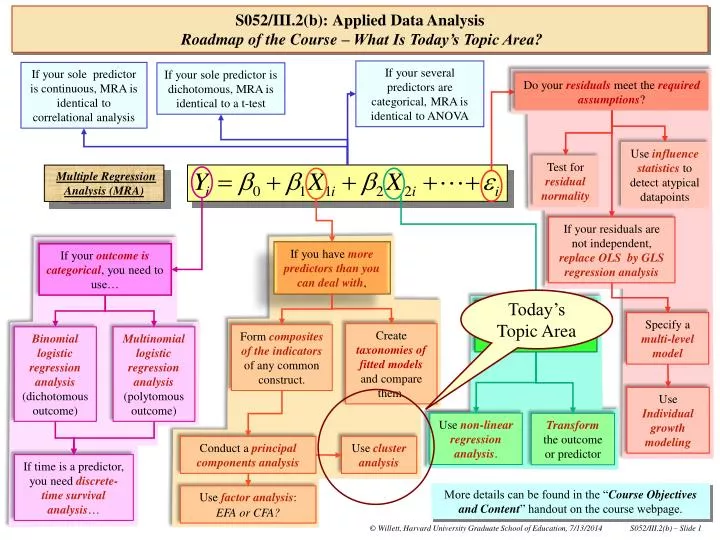
If your several predictors are categorical, MRA is identical to ANOVA If your sole predictor is continuous, MRA is identical to correlational analysis If your sole predictor is dichotomous, MRA is identical to a t-test Do your residuals meet the requiredassumptions? Use influence statistics to detect atypical datapoints Test for residual normality Multiple Regression Analysis (MRA) If your residuals are not independent, replace OLS byGLS regression analysis If you have more predictors than you can deal with, If your outcome is categorical, you need to use… If your outcome vs. predictor relationship isnon-linear, Today’s Topic Area Specify amulti-level model Create taxonomies of fitted models and compare them. Form composites of the indicators of any common construct. Binomiallogistic regression analysis (dichotomous outcome) Multinomial logistic regression analysis (polytomous outcome) Use Individual growth modeling Use non-linear regression analysis. Transform the outcome or predictor Conduct a principal components analysis Use cluster analysis If time is a predictor, you need discrete-time survival analysis… More details can be found in the “Course Objectives and Content” handout on the course webpage. S052/III.2(b):Applied Data AnalysisRoadmap of the Course – What Is Today’s Topic Area? Use factor analysis: EFA or CFA?
Yasgur’s Farm, Woodstock, NY, August 15, 1967 S052/III.2(b): Exploratory Cluster Analysis of PeoplePrinted Syllabus – What Is Today’s Topic? Please check inter-connections among the Roadmap, the Daily Topic Area, the Printed Syllabus, and the content of today’s class when you pre-read the day’s materials. Why Conduct Cluster Analyses of People? (Slide 3). A Simple Eyeball Cluster Analysis, To Establish the Basic Principles (Slide 4-13). More Complex Example of Cluster Analysis, w/ Additional Statistical Supports and Tools (Slide 14-22). Using the Cluster Analysis of People to Detect Multivariate Outliers (Slide 23-27).
S052/III.2(b): Exploratory Cluster Analysis of PeopleWhy Conduct Cluster Analyses of People? • We have clustered variables, in our previous class, but individuals can also be clustered into homogeneous groups – useful for: • Data exploration, • Hypothesis generation, • Creating typologies and taxonomies, • … • Two examples today: • A cluster analysis of college freshmen, based on measures of their academic comfort and introversion/extroversion. • A cluster analysis of teachers, based on their self-reported efficacy. A simple limited example –small sample, limited number of measures – essentially, an “eyeball cluster analysis of college freshmen” that serves to introduce the basic ideas of thecluster analysis of individuals. A more realistic complex example – larger sample, eight measures -- that will serve to introduce more-advanced cluster-analytic strategies & reveal some of the dangers implicit in the analysis.
S052/III.2(b): Exploratory Cluster Analysis of PeopleA Simple Eyeball Cluster Analysis, To Establish the Basic Principles RQ: Are There Natural And Distinct Groupings Of Freshmen In The Sample, Within Which Freshman Are Homogeneous On Academic Comfort And Introversion/Extroversion?
S052/III.2(b): Exploratory Cluster Analysis of PeopleA Simple Eyeball Cluster Analysis, To Establish the Basic Principles Data Analytic Handout III.2(b).1… STATA programming code: Usual data input & labeling statements *------------------------------------------------------------------------ * Input raw dataset, name and label variables and selected values. *------------------------------------------------------------------------ * Input the target dataset: infile ID AC IE using "C:\My Documents\ … \Datasets\SCII.txt" * Label the variables: label variable ID "Subject ID" label variable AC "Academic Comfort" label variable IE "Introversion-Extroversion" *------------------------------------------------------------------------ * Obtain preliminary descriptive statistics *------------------------------------------------------------------------ * List the cases in the dataset: list ID AC IE * Obtain univariate descriptive statistics on two dimensions of behavior: tabstat AC IE, statistics(n mean sd min max) columns(statistics) *------------------------------------------------------------------------ * Perform an "eyeball" cluster analysis *------------------------------------------------------------------------ * Plot participants in space defined by academic comfort & introversion: graph twoway scatter AC IE , msymbol(+) name(III_2b_1_g1,replace) *------------------------------------------------------------------------ * Perform a standard cluster analysis *------------------------------------------------------------------------ * Choose Euclidean geometry & avg linkage method, obtain tree diagram: cluster averagelinkage AC IE, measure(Euclidean) name(collkids) cluster dendrogram collkids, label(ID) title(Tree Diagram) /// ytitle(Euclidean Distance) xtitle(Freshman ID) /// name(III_2b_1_g2,replace) Inspect the data and obtain descriptive statistics on academic comfort, AC, & introversion/extroversion, IE. Conduct aneyeball cluster analysisby listing out the freshmen and inspecting their distribution in the “space” defined by academic comfort, AC, & introversion/extroversion, IE. Choose Euclideangeometry and the “average” method of measuring distancesbetween clusters Conduct an automated cluster analysis of the data using cluster, Label the cluster solution “collkids” Produce a tree plotor dendrogram of the “collkids” cluster solution
S052/III.2(b): Exploratory Cluster Analysis of PeopleA Simple Eyeball Cluster Analysis, To Establish the Basic Principles Here are thedataand ascatterplot of the freshman in a two-dimensional space defined by AC and IE… But, clearly, there is no single “answer” to the question “What is the natural grouping?” ID AC IE 1 39 71 2 36 34 3 13 56 4 50 44 5 34 40 6 76 49 7 21 64 8 15 57 9 15 66 10 23 63 11 11 56 12 36 61 13 36 62 14 58 52 15 58 40 16 41 60 17 53 50 18 41 39 19 44 37 20 43 40 80 ˆ ‚ * ‚ A ‚ c ‚ a ‚ d ‚ e 60 ˆ m ‚ * * i ‚ * c ‚ * ‚ C ‚ o ‚ * * m 40 ˆ * * * f ‚ * * * o ‚ * r ‚ t ‚ ‚ S ‚ * c 20 ˆ * o ‚ r ‚ * * * e ‚ * ‚ ‚ ‚ 0 ˆ ‚ Šˆƒƒƒƒƒƒƒƒƒƒƒƒƒˆƒƒƒƒƒƒƒƒƒƒƒƒƒˆƒƒƒƒƒƒƒƒƒƒƒƒƒˆƒƒƒƒƒƒƒƒƒƒƒƒƒˆƒƒƒƒƒƒƒƒƒƒƒƒƒˆ 30 40 50 60 70 80 Introversion-Extraversion Score A hierarchy of solutions exists, each nested within the next one. Issues? • Can we persuade a computer to recognize all the nested solutions? • How do we chooseamong the many nested cluster solutions, to find the “best”? • Does it make sense to even think there might be a “best” cluster solution? Inspecting the plot, your eye is drawn to the natural grouping of individuals in the data
Student #17 53 (53 - 34) = 19 34 (50 - 40) = 10 Student #5 50 40 S052/III.2(b): Exploratory Cluster Analysis of PeopleA Simple Eyeball Cluster Analysis, To Establish the Basic Principles Here’s one clustering algorithm we could use … • Treat the region spanned by the clustering variables (here, AC & IE) as defining a “space”: • Plot all cases as “objects” in this space. • Start with each objectas its own cluster: • Here, we start with 20 clusters. • Compute the “distance” between each object and every other one, using a sensible algorithm… 80 ˆ ‚ * ‚ A ‚ c ‚ a ‚ d ‚ e 60 ˆ m ‚ * * i ‚ * c ‚ * ‚ C ‚ o ‚ * * m 40 ˆ * * * f ‚ * * * o ‚ * r ‚ t ‚ ‚ S ‚ * c 20 ˆ * o ‚ r ‚ * * * e ‚ * ‚ ‚ ‚ 0 ˆ ‚ Šˆƒƒƒƒƒƒƒƒƒƒƒƒƒˆƒƒƒƒƒƒƒƒƒƒƒƒƒˆƒƒƒƒƒƒƒƒƒƒƒƒƒˆƒƒƒƒƒƒƒƒƒƒƒƒƒˆƒƒƒƒƒƒƒƒƒƒƒƒƒˆ 30 40 50 60 70 80 Introversion-Extraversion Score
S052/III.2(b): Exploratory Cluster Analysis of PeopleA Simple Eyeball Cluster Analysis, To Establish the Basic Principles Here’s one clustering algorithm we could use … • Rankthe pairwise distances, pick the two closest objects, call them a cluster: • Here, the first cluster formed contains objects #12 & #13. • Replace the objects within the new cluster by a single object to represent them all: • There are now 19 objects remaining. • Repeat interminably. Re-compute the pair-wise distances among remaining objects, re-rank the distances, pick the pair of objects now separated by the new shortest distance, call them the next cluster, thereby reducing the number of objects again by one. • Continue untilall objects end up in a single super-cluster that contains all objects. • Find a way to plot and inspect the cluster solution. 80 ˆ ‚ * ‚ A ‚ c ‚ a ‚ d ‚ e 60 ˆ m ‚ * * i ‚ * c ‚ * ‚ C ‚ o ‚ * * m 40 ˆ * * * f ‚ * * * o ‚ * r ‚ t ‚ ‚ S ‚ * c 20 ˆ * o ‚ r ‚ * * * e ‚ * ‚ ‚ ‚ 0 ˆ ‚ Šˆƒƒƒƒƒƒƒƒƒƒƒƒƒˆƒƒƒƒƒƒƒƒƒƒƒƒƒˆƒƒƒƒƒƒƒƒƒƒƒƒƒˆƒƒƒƒƒƒƒƒƒƒƒƒƒˆƒƒƒƒƒƒƒƒƒƒƒƒƒˆ 30 40 50 60 70 80 Introversion-Extraversion Score
Start, with 20 clusters S052/III.2(b): Exploratory Cluster Analysis of PeopleA Simple Eyeball Cluster Analysis, To Establish the Basic Principles Finish, with 1 cluster Question: Out Of All These Possibilities, What Is The Single “Ideal” Cluster Solution?
Once all objects closer than 32have combined, only two clusters remain, with case #6 having finally joined another cluster Once all objects closer than 23have combined, there are only threeclusters – including the case #6 singleton. Once all objects closer than 11have clustered, there are five clusters remaining – including one that contains only case #6 (an outlier?). S052/III.2(b): Exploratory Cluster Analysis of PeopleA Simple Eyeball Cluster Analysis, To Establish the Basic Principles
Cluster analysis and dendrogram, as before … List out the values of the original variables and the new cluster-membership variable, for inspection. Characterize the two selected clustersby examining the profile of meanson the original variables, by cluster S052/III.2(b): Exploratory Cluster Analysis of PeopleA Simple Eyeball Cluster Analysis, To Establish the Basic Principles Inspecting a two-cluster solution … Data Analytic Handout III.2(b).2 *-------------------------------------------------------------------------------- * Perform a standard cluster analysis *-------------------------------------------------------------------------------- * Choose Euclidean geometry & average linkage method, obtain tree diagram: cluster averagelinkage AC IE, measure(Euclidean) name(collkids) cluster dendrogram collkids, label(ID) /// title(Tree Diagram) /// ytitle(Euclidean Distance) xtitle(Freshman ID) /// name(III_2b_1_g2,replace) *-------------------------------------------------------------------------------- * Select a two-cluster solution as the "ideal" solution *-------------------------------------------------------------------------------- * Create a new variable "clustermem" to record into which of the final two * clusters each freshman is grouped: cluster generate clustermem = groups(2), name(collkids) * Sort the freshmen by their cluster membership, and list the data for inspection: sort clustermem list ID AC IE clustermem *-------------------------------------------------------------------------------- * Display and summarize descriptive details of the two cluster solution. *-------------------------------------------------------------------------------- * Plot the participants in the AC/IE space, and label them by cluster membership: graph twoway scatter AC IE, /// msymbol(i) mlabel(clustermem) mlabposition(0) /// name(III_2b_2_g1,replace) * Obtain descriptive statistics on AC and IE, by cluster membership: tabstat AC IE, by(clustermem) statistics(mean n) • Take the “collkids” cluster solution: • Pick a “two-cluster” solution as ideal, using the “groups(2)” option. • Then, “generate” a new variable – clustermem -- to record which cluster each freshman is a member of. Inspect the distribution ofcluster membershipin the two-dimensional space defined by the original variables
Two major clusters of freshmen Notice this new variable called clustermemhas appeared in the dataset – used for classifying cases into clusters in subsequent analysis S052/III.2(b): Exploratory Cluster Analysis of PeopleA Simple Eyeball Cluster Analysis, To Establish the Basic Principles +-------------------------+ | ID AC IE cluste~m | |-------------------------| | 9 15 66 1 | | 11 11 56 1 | | 13 36 62 1 | | 7 21 64 1 | | 3 13 56 1 | |-------------------------| | 16 41 60 1 | | 8 15 57 1 | | 12 36 61 1 | | 1 39 71 1 | | 10 23 63 1 | |-------------------------| | 19 44 37 2 | | 15 58 40 2 | | 6 76 49 2 | | 20 43 40 2 | | 18 41 39 2 | |-------------------------| | 4 50 44 2 | | 14 58 52 2 | | 5 34 40 2 | | 17 53 50 2 | | 2 36 34 2 | +-------------------------+
S052/III.2(b): Exploratory Cluster Analysis of PeopleA Simple Eyeball Cluster Analysis, To Establish the Basic Principles clustermem | AC IE -----------+-------------------- 1 | 25 61.6 | 10 10 -----------+-------------------- 2 | 49.3 42.5 | 10 10 -----------+-------------------- Total | 37.15 52.05 | 20 20 -------------------------------- Second Clusterof freshmen consists of students for whom: Academic Comfort = moderately high Introversion = lower This group prefers to work with people, not things, and is reasonably comfortablein the academic environment First Clusterof freshmen consists of students for whom: Academic Comfort = low Introversion = high This group prefers to work with things, not people, and is uncomfortable with the academic environment
S052/III.2(b): Exploratory Cluster Analysis of PeopleMore Complex Example of the Cluster Analysis of People
Usual data input steps Here, I created standardized versions of each original variable. (I did this for two reasons: (a) to illustrate how to standardize variables, in STATA, and (b) I was having trouble with “ties” in the original data). Create the dendrogram, showing only the last 50 “objects” (i.e., clusters of teachers) in the tree, because it is so complex. Conduct the cluster analysis – again using Euclidean geometry and average linkage -- and name the cluster solution Teachers. S052/III.2(b): Exploratory Cluster Analysis of PeopleMore Complex Example of the Cluster Analysis of People * Input the raw dataset, standardize the variables and label. *---------------------------------------------------------------------------- * Input the target dataset: • infile TEACHID SCHID EFFT EFFCM EFFAM EFFDIFF EFFPD EFFLRN /// EFFCUR EFFGOOD AGE MALE HISCHOOL WHITE BLACK HISP ASIAN PCTFRL /// using "C:\My Documents\My Course Stuff\ … \Datasets\EFFICACY.txt" * Standardize variables describing teacher efficacy, to mean 0 & st. dev. 1; egens_EFFT = std(EFFT) egens_EFFCM = std(EFFCM) egens_EFFAM = std(EFFAM) egens_EFFDIFF = std(EFFDIFF) egens_EFFPD = std(EFFPD) egens_EFFLRN = std(EFFLRN) egens_EFFCUR = std(EFFCUR) egens_EFFGOOD = std(EFFGOOD) * Label newly standardized variables describing teacher efficacy; label vars_EFFT "I am effective in teaching students" label vars_EFFCM "I manage my classroom & maintain discipline" label vars_EFFAM "I interact effectively with students families" label vars_EFFDIFF "I am making a difference to my students" label vars_EFFPD "I am learning continuously on the job" label vars_EFFLRN "My students learn what I teach" label vars_EFFCUR "I find it easy to cover the material" label vars_EFFGOOD "I am doing a good job for my students“ *--------------------------------------------------------------------------- * Conduct an initial cluster analysis & inspect dendrogram *--------------------------------------------------------------------------- * Cluster teachers using average linkage method and Euclidean geometry, * calling the stored cluster solution by the name "Teachers": cluster averagelinkages_EFFTs_EFFCMs_EFFAMs_EFFDIFFs_EFFPD /// • s_EFFLRNs_EFFCURs_EFFGOOD, measure(Euclidean) name(Teachers) * Obtain tree-diagram of cluster solution "Teachers," displaying clustering * of only the last 50 objects in the cluster solution: cluster dendrogram Teachers, cutnumber(50) /// title(Tree Diagram/Teacher Efficacy) /// ytitle(Euclidean Distance) xtitle(Teacher ID) /// name(III_2b_3_g1,replace) Cluster analysis conducted inData Analytic Handout III.2(b).3 …
Introducing the pseudo-F statistic: • • • • • • • • High F • • • • • • Low F • • To identify exceptional cluster structure, we are seeking those specific steps in the cluster history where the value of the pseudo-F statisticis unexpectedly high S052/III.2(b): Exploratory Cluster Analysis of PeopleMore Complex Example of the Cluster Analysis of People
First, I invoked the “cluster stop” command with respect to the “Teachers” cluster solution that I had obtained earlier. The “stop” command is asking for the Pseudo-F statistics (“Calinski”) to be computed for cluster solutions 2 thru 50. The results are stored in a matrix that I have named “history.” Then, I took the “history” matrix and renamed two of its columns, as new variables. I chose the columns that contained the number of clusters (nclusters) and the pseudo-F statistic (pseudoF) , at each step. Then, I requested a two-way scatterplot of the Pseudo-F statistic versus the number of clusters at each step. S052/III.2(b): Exploratory Cluster Analysis of PeopleMore Complex Example of the Cluster Analysis of People I estimated the pseudo-F statistic inData Analytic Handout III.2(b).3 … *------------------------------------------------------------------------------- * Generate/display pseudo-F stats to help select a particular cluster solution *------------------------------------------------------------------------------- * Output details of cluster solution into a "history" matrix that summarizes the * distinctness of the cluster solution, at each step. Higher values of the * pseudo-F statistic indicate a more distinct, or "tighter," set of clusters. cluster stop Teachers, rule(calinski) groups(2/50) matrix(history) * Convert the columns of the cluster history matrix into variables, and rename: svmat history rename history1 nclusters rename history2 pseudoF * Plot the values of the pseudo-F statistic by the number of clusters, at each * step, for inspection: graph twoway scatter pseudoFnclusters, /// msymbol(+) connect(l) lpattern(-) /// ytitle(Pseudo-F Statistic) xtitle(Number of Clusters Present) /// name(III_2b_1_g2,replace)
8 clusters 34 clusters 49 clusters 17 clusters 2 clusters S052/III.2(b): Exploratory Cluster Analysis of PeopleMore Complex Example of the Cluster Analysis of People +---------------------------+ | | Calinski/ | | Number of | Harabasz | | clusters | pseudo-F | |-------------+-------------| | 2 | 23.16 | | 3 | 18.92 | | 4 | 16.10 | | 5 | 12.73 | | 6 | 10.68 | | 7 | 9.23 | | 8 | 29.65 | | 9 | 27.40 | | 10 | 24.58 | | 11 | 22.97 | | 12 | 21.04 | | 13 | 19.86 | | 14 | 18.67 | | 15 | 18.05 | | 16 | 16.99 | | 17 | 29.02 | | 18 | 28.64 | | 19 | 27.18 | | 20 | 25.95 | | 21 | 24.82 | | 22 | 25.27 | | 23 | 25.11 | | 24 | 24.82 | | 25 | 24.08 | | 26 | 23.60 | | 27 | 22.93 | | 28 | 22.77 | | 29 | 22.54 | | 30 | 22.17 | | 31 | 21.52 | | 32 | 20.92 | | 33 | 20.60 | | 34 | 23.39 | … … … | 48 | 19.24 | | 49 | 22.69 | | 50 | 22.38 | +---------------------------+
2 cluster solution 8 cluster solution 17 cluster solution S052/III.2(b): Exploratory Cluster Analysis of PeopleMore Complex Example of the Cluster Analysis of People
Adopt the 8-cluster solution as “ideal” & and create a new variable called clustermem to contain each teacher’s cluster membership. List the cluster membership of a few teachers for inspection Estimate, and inspect, the means of the efficacy indicators within the two most populous clusters S052/III.2(b): Exploratory Cluster Analysis of PeopleMore Complex Example of the Cluster Analysis of People Interpretation of the obtained cluster solution … *------------------------------------------------------------------------- * Focus on eight-cluster solution as an "ideal" solution, and inspect it *------------------------------------------------------------------------- * Adopt eight-cluster solution as "best" and create a new variable called * "clustermem" to record which cluster each teacher is a member of: cluster generate clustermem = groups(8), name(Teachers) * List sub-sample of teachers, for inspection of their cluster membership: sort TEACHID list TEACHID clustermem in 1/40 * Obtain frequency of teachers in each cluster, so we can see if some * are more populous than others: tabstat TEACHID, by(clustermem) statistics(n) * Focus on two most populous clusters, and obtain descriptive statistics * on teacher efficacy within them, by cluster membership: tabstat EFFT-EFFGOOD if clustermem<=2, /// clustermem) statistics(mean) format(%3.1f) clustermem | N -----------+---------- 1 | 372 2 | 78 3 | 1 4 | 2 5 | 2 6 | 1 7 | 2 8 | 1 -----------+---------- Total | 459 ----------------------
First Cluster (n=372) • On average, these report higher levels of efficacy on every indicator, except EFFCUR. • They are generally happy about the job they do except that they find it less easy to cover the material in the curriculum than their peers in the second cluster. • Second Cluster (n=78) • On average, these teachers have levels of efficacy that are about one unit lower across all eight measures, except EFFCUR. • On this latter indicator, they are more confident about covering the curricular material that their peers in the first cluster. S052/III.2(b): Exploratory Cluster Analysis of PeopleMore Complex Example of the Cluster Analysis of People Table III.2(b).4. Within-cluster sample averages of eight indicators of teacher efficacy, by membership in the two most populous clusters.
Conduct PCAof the 8 efficacy measures to reduce their dimensionality, in service of the subsequent plotting of the obtained cluster solution. Output composite scores on the first three principal components, EFFIC_1 thru EFFIC_3 Plot, and label, teacher membership in the two most populous clusters in the space defined by the first three principal components Do it again, with a different spatial orientation You can tilt and rotate the plot to your heart’s desire scat3 provides a three-dimensional scatter plot, with EFFIC_1scores on the vertical axis S052/III.2(b): Exploratory Cluster Analysis of PeopleMore Complex Example of the Cluster Analysis of People Visualizing the spatial separation of the two largest clusters … *-------------------------------------------------------------------------------- * Display final cluster membership in the space defined by teacher efficacy *-------------------------------------------------------------------------------- * You cannot plot cluster membership in the eight-dimensional space defined * by the indicators of teacher efficacy, as the plot is too complex. But you can * first reduce dimensionality from 8 down to 3 sensibly, using PCA, as follows: pcaEFFT-EFFGOOD predict EFFIC_1 EFFIC_2 EFFIC_3, score * Then, plot the obtained cluster membership for the first two (and largest) * clusters in space defined by the first, second & third principalcomponents: * Plot #1: scat3 EFFIC_3 EFFIC_2 EFFIC_1 if clustermem<=2, /// axistype(minimum) /// rotate(60) elevate(15) /// titlex(EFFIC_1) titley(EFFIC_2) titlez(EFFIC_3) /// spikes(vertical lwidth(vvthin) lcolor(emerald)) /// msymbol(i) mlabel(clustermem) mlabposition(0) /// name(III_2b_3_g3,replace) * Plot #2: scat3 EFFIC_3 EFFIC_2 EFFIC_1 if clustermem<=2, /// axistype(minimum) /// rotate(60) elevate(65) /// titlex(EFFIC_1) titley(EFFIC_2) titlez(EFFIC_3) /// spikes(vertical lwidth(vvthin) lcolor(emerald)) /// msymbol(i) mlabel(clustermem) mlabposition(0) /// name(III_2b_3_g4,replace)
S052/III.2(b): Exploratory Cluster Analysis of PeopleMore Complex Example of the Cluster Analysis of People Are there really two major clusters, or is it really one cluster that’s been “artificially” sliced into two?
Inspecting the ACvs. IE scatter-plot, you are struck by the placement of Freshman #6 as a potential oddityin the point cloud. Perhaps the most effective use of the cluster analysis of people is in the detection of multivariate outliers … recall the data from our example of freshman academic comfort and introversion/extroversion … 80 ˆ ‚ * ‚ A ‚ c ‚ a ‚ d ‚ e 60 ˆ m ‚ * * i ‚ * c ‚ * ‚ C ‚ o ‚ * * m 40 ˆ * * * f ‚ * * * o ‚ * r ‚ t ‚ ‚ S ‚ * c 20 ˆ * o ‚ r ‚ * * * e ‚ * ‚ ‚ ‚ 0 ˆ ‚ Šˆƒƒƒƒƒƒƒƒƒƒƒƒƒˆƒƒƒƒƒƒƒƒƒƒƒƒƒˆƒƒƒƒƒƒƒƒƒƒƒƒƒˆƒƒƒƒƒƒƒƒƒƒƒƒƒˆƒƒƒƒƒƒƒƒƒƒƒƒƒˆ 30 40 50 60 70 80 Introversion-Extraversion Score S052/III.2(c): Selected Multivariate Data-Analytic MethodsUsing Cluster Analysis of People To Detect Multivariate Outliers ID AC IE 1 39 71 2 36 34 3 13 56 4 50 44 5 34 40 6 76 49 7 21 64 8 15 57 9 15 66 10 23 63 11 11 56 12 36 61 13 36 62 14 58 52 15 58 40 16 41 60 17 53 50 18 41 39 19 44 37 20 43 40
Finish, with 1 cluster Freshman #6 remains a singleton until almost the end of the cluster analysis, when he finally joins together with an existing cluster This phenomenon suggests that the cluster analysis of individuals may be an effective way of detecting “multivariate outliers” Start with 20 clusters The atypical placement of this person in the AC vs. IE space is also reflected in the cluster solution…. S052/III.2(c): Selected Multivariate Data-Analytic MethodsUsing Cluster Analysis of People To Detect Multivariate Outliers
Here’s an example of this, using the teacher satisfaction data … Handout III.2(c).1 *------------------------------------------------------------------------------- * Conduct an initial cluster analysis *------------------------------------------------------------------------------- * Cluster the teachers using the average linkage method and Euclidean geometry, * calling the stored cluster solution by the name "Teachers": cluster averagelinkages_EFFTs_EFFCMs_EFFAMs_EFFDIFFs_EFFPDs_EFFLRN /// s_EFFCURs_EFFGOOD, measure(Euclidean) name(Teachers) *------------------------------------------------------------------------------- * Select a solution with additional clusters beyond the populated clusters *------------------------------------------------------------------------------- * Adopt 8-cluster solution and create the new variable "clustermem" to record * into which of the eight clusters each teacher is grouped: cluster generate clustermem = groups(8), name(Teachers) label variable clustermem "Cluster Membership" * Obtain frequency of teachers in each cluster: tabstat TEACHID, by(clustermem) statistics(n) * Examine teachers in the depopulated clusters, as they are the "unique" ones. sort clustermem list clustermem TEACHID EFFT-EFFGOOD if clustermem>=3 & clustermem<=8, /// noobssepby(clustermem) cluster dendrogram Teachers, cutnumber(20) label(clustermem) /// title(Tree Diagram/Teacher Efficacy) /// ytitle(Euclidean Distance) xtitle(Teacher ID) /// name(III_2c_1_g1,replace) S052/III.2(c): Selected Multivariate Data-Analytic MethodsUsing Cluster Analysis of People To Detect Multivariate Outliers Conduct the standard cluster analysis Focus on a cluster solution, with a larger number of clusters, Display the number of participants in each cluster List the values of the indicators for teachers in the depopulated clusters Provide a dendrogram, showing the depopulated clusters
S052/III.2(c): Selected Multivariate Data-Analytic MethodsUsing Cluster Analysis of People To Detect Multivariate Outliers One of these things is not like the others? Notice that, after thousands of steps in the cluster history, clusters #3, #6 and #8 each contain a single (odd-ball) teacher, almost all of the way to the end? clustermem | N -----------+---------- 1 | 372 2 | 78 3 | 1 4 | 2 5 | 2 6 | 1 7 | 2 8 | 1 -----------+---------- Total | 459 ---------------------- This suggests that these three teachers are “very remote” from everyone else in the dataset – that is, they are potential multivariate outliers
Let’s find out who the outlying cases are, and how they responded on the 6 indicators of efficacy… +-----------------------------------------------------------------------------------------+ | cluste~m TEACHID EFFT EFFCM EFFAM EFFDIFF EFFPD EFFLRN EFFCUR EFFGOOD | |-----------------------------------------------------------------------------------------| | 3 4402 5 6 6 6 2 4 2 6 | |-----------------------------------------------------------------------------------------| | 6 15606 2 4 1 3 5 4 6 2 | |-----------------------------------------------------------------------------------------| | 8 12101 4 3 5 5 1 4 6 2 | +-----------------------------------------------------------------------------------------+00 S052/III.2(c): Selected Multivariate Data-Analytic MethodsUsing Cluster Analysis of People To Detect Multivariate Outliers They are strange and conflicted teachers indeed, perhaps even data-coding errors …