Download
1 / 56
590 likes | 915 Views
Layered Graph Drawing (Sugiyama Method). Drawing Conventions and Aesthetics. a digraph. A possible layered drawing. The Sugiyama method. Layered networks are often used to represent dependency relations. Sugiyama et al. developed a simple method for drawing layered networks in 1979.

E N D
Drawing Conventions and Aesthetics a digraph A possible layered drawing
The Sugiyama method • Layered networks are often used to represent dependency relations. • Sugiyama et al. developed a simple method for drawing layered networks in 1979. • Sugiyama’s aims included: • few edge crossings • edges as straight as possible • nodes spread evenly over the page • The Sugiyama method is useful for • dependency diagrams • flow diagrams • conceptual lattices • other directed graphs: acyclic or nearly acyclic.
The Sugiyama method • Step 1Cycle Removal • Step 2Layering
The Sugiyama method • Step 1Cycle Removal • Step 2Layering • Step 3Node ordering
The Sugiyama method • Step 1Cycle Removal • Step 2Layering • Step 3Node ordering • Step 4Coordinate assignment
Layered Drawing of Digraphs • Polyline drawings of digraphs with vertices arranged in horizontal layers • Sugiyama, Tagawa and Toda ‘81 • Eades and Sugiyama ‘91 • Evolutionary algorithm approach of Branke et al. • Magnetic field approach of Sugiyama and Misue. • Attractive in practice: most graph drawing systemsinclude the Sugiyama method.
Step 1. Cycle Removal • Input graph may contain cycles 1. make an acyclic digraph by reversing some edges 2. draw the acyclic graphs 3. render the drawing with the original edge directions Acyclic graph by reversing two edges
Step 1. Cycle Removal • Each cycle must have at least one edge against the flow • We need to keep the number of edges against the flow small • Main problem: how to choose the set of edges R so that it is small • Feedback arc set: • set of edges R whose reversing makes the digraph acyclic • Feedback edge set: • set of edges whose removal makes the digraph acyclic • Maximum acyclic subgraph problem • find a maximum set Ea such that the graph(V, Ea) contains no cycles : NP-hard • Feedback arc set problem • find a minimum set Ef such that the graph(V, E \ Ef) contains no cycles : NP-hard
Step 1. Cycle Removal • Edges in E \ Ea will be reversed • Assume no two-cycles (or delete both two edges) • Heuristics • Fast heuristic • Enhanced Greedy heuristic • Randomized algorithm:[BS90]: O(mn) time • Exact algorithm: [Grotschel et al 85, Reinelt 85]
1. Fast heuristic • Maximum acyclic subgraph problem • equivalent to unweighted linear ordering problem: find an ordering of the vertices, a mapping o such that the # of edges (u,v), o(u) > o(v) is minimized. • Easiest heuristic • take an arbitrary ordering • then delete the edges (u,v) with o(u) > o(v) • May use given ordering: BFS or DFS • No performance guarantee: reverse |E|-|V|-1 edges (DFS) • Heuristic that guarantees acyclic set of size at least ½|E| [BS90] • Delete for every vertex either incoming or outgoing edges • Linear time
2. Enhanced greedy heuristic • Feedback set problem: equivalent to finding a vertex sequence with as few leftward edges as possible • S=(v1, v2, …, vn): vertex sequence of a digraph G • Leftward edge: (vi, vj) with i > j • set of leftward edges for a vertex sequence forms a feedback set
Greedy Cycle Removal • Greedy cycle removal heuristic [Eades et al 93] • Source & sink play a special role: edges incident to source & sink cannot be part of a cycle • Successively remove vertices from G • Add each in turn, to one of two lists Sl & Sr, either the end of Sl or the beginning of Sr • Greedy: choice of vertices to be removed and the choice of the list to be added
Greedy Cycle Removal • Greedy Cycle Removal [Eades et al 93] • All sinks (sources) should be added to Sr (Sl) • Choose a vertex u whose outdeg(u)-indeg(u) is maximized and add to Sl • performance • Can be implemented in linear time and space • Sparse graph: Ea with at least 2/3|E|
Analysis • Delete all two cycles before applying Greedy-cycle-removal • Two-cycle: a directed cycle with two edges • [Theorem] G: connected digraph with n vertices & m edges without two cycles. Greedy-Cycle-Removal computes a vertex sequence S of G with at most m/2 – n/6 leftward edges • [Theorem] Greedy-Cycle-Removal can be implemented in linear time & space • Simple & speedy • Sparse graph [EL95] [Theorem] G: connected digraph with n vertices & m edges without two cycles. Each vertex of G has total degree at most 3. Greedy-Cycle-Removal computes a vertex sequence S of G with at most m/3 leftward edges
Step 2. Layer Assignment • Layering: partition V into L1, L2, …, Lh • Layered (di)graph: digraph with layers • Height h: # of layers • H-layered graph: digraph with height h • Width w: # of vertices with largest layer • Span of an edge • Proper digraph: no edge has a span > 1 • Some application, vertices are preassigned to layers • However, in most applications, we need to transform an cyclic digraph into a layered digraph
Y=4 Y=3 Y=2 Y=1 Layering Introducing dummy vertices
Step 2. Layer Assignment • Requirements 1. Layered digraph should be compact: height & width 2. The layering should be proper: add dummy vertices 3. The number of dummy vertices should be small A. time depends on the total number of vertices B. bends in the final drawing occur only at dummy vertices C. the number of dummy vertices on an edge measures the y extent of the edge: avoid long edge. • Methods 1. Longest path layering: minimize height 2. Layering to minimize width 3. Minimize the number of dummy vertices
Three Layering Algorithms • Longest Path • Coffman-Graham • Network Simplex Grafo1012 (Di Battista et al., Computational Geometry: Theory and Applications, (7), 1997)
Coffman-Graham Layering (1972) h (2-2/W)hopt
ILP formulation Network Simplex Layering (AT&T, 1993)
1. Longest path layering • Minimizing the height • Place all sinks in layer L1 • Each remaining vertex v is placed in layer Lp+1, where the longest path from v to a sink has length p • Can be computed in linear time • Main drawback: too wide
2. Layering to minimize width • Finding a layering with minimum height subject to a maximum width constraint: Precedence-constrained multiprocessor scheduling problem -> NP-complete [GJ79] • Coffman-Graham Layering • Input: reduced graph G (no transitive edges) and W • Output: layering of G with width at most W • Aim: ensure the height of the layering is kept small [LS77] • Two phases 1. Order the vertices 2. Assign layers • Width: does not count dummy vertices
Coffman-Graham Layering • Simple lexicographic order: • First phase: lexicographical ordering • Second phase: ensure that no layer receive more than W vertices • [LS77] height is not too large
3. Minimizing # of dummy vertices • one can compute a layering in polynomial time that minimizes the number of dummy vertices [GKNV93] • f = S (u,v)V ( y(u) - y(v) - 1) • f: sum of vertical spans of the edges in the layering - # of edges : (# of dummy vertices) • Layer assignment problem is reduced to choosing y-coordinates to minimize f • Integer linear programming problem
Remark • Methods 1. Layering for general graphs [Sander 96] 2. Minimizing the height: Longest path layering 3. Layering with given width: Coffman-Graham algorithm: width is more important than height 4. Minimizing the total edge span (# of dummy vertices) : relatively compact drawing • [Sander 96] 1. Calculate y by DFS or BFS 2. Calculate minimum cost spanning trees 3. Apply spring embedder
Step 3. Crossing Reduction • Input: proper layered graph • # of edge crossings does not depend on the precise position of the vertices, but only the ordering of the vertices within each layer (combinatorial, rather than geometric) • NP-complete, even for only two layers [GJ83] • Many heuristics • Layer-by-layer sweep: two layer crossing problem • 1. Sorting • 2. Barycenter method • 3. Median method • 4. Integer programming method: exact algorithm
1 2 2 1 3 4 5 3 4 5 6 6 7 7 step 3 8 9 9 8 10 11 12 10 12 11 13 13 14 14 5 edge crossings Crossing Reduction: ordering 21 edge crossings
Layer-by-layer sweep • A vertex ordering of layer L1 is chosen • For i = 2, 3, …, h • The vertex ordering of Li-1 is fixed • Reordering the vertices in layer Li to reduce edges crossings between Li-1 and Li • Two layer crossing problem: given a fixed ordering of Li-1, choose a vertex ordering of Layer Li to minimize # of crossings • Several variations: layer-by-layer sweep
free free free fixed fixed fixed Layer-by-layer sweep • Step 3 uses a “layer-by-layer sweep”, from bottom to top. • At each stage of the sweep, we: • hold one layer fixed, and • Re-arrange the nodes in the layer above to avoid edge crossings. 1 2 L6 3 4 L5 5 6 7 L4 L3 8 9 10 11 L2 12 L1 13 14
L3 8 9 free L2 fixed 10 11 12 ? 9 8 L3 10 L2 11 12 Two layer crossing problem The difficult part is to re-arrange the free layer 1 2 3 4 5 6 7 L3 8 9 free fixed 10 L2 11 12 13 14
6 1 2 Li+1 free fixed 3 8 5 9 4 7 Li Two layer crossing problem • The problem of finding an optimal solution is NP-hard. • Heuristics • Barycenter method: place each free node at the barycenter of its neighbours. • Median method: place each free node at the median of its neighbours.
Two layer crossing problem • given a two-layered digraph G=(L1,L2,E) and an ordering x1 of L1, find an ordering x2 of L2, such that cross(G,x1,x2) = opt(G,x1) • two-layered digraph G=(L1, L2, E): a bipartite digraph • cross(G, x1, x2): # of crossings in a drawing of G • opt(G,x1): min x2 cross(G, x1, x2) • NP-complete: [EW94] • Simple observation: u and v are in L2 the # of crossings between edges incident with u and edges incident with v depends only on the relative positions of u and v and not on the other vertices
Crossing number • Crossing number cuv • # of crossings that edges incident to u make with edges incident v, when x2(u) < x2(v) • # of pairs (u,w), (v,z) of edges with x1(z) < x1(w)
1. Sorting Method • Aim: to sort the vertices in L2 into an order that minimizes # of crossings • Naive algorithm: O(|E|)2, can be reduced • Adjacent-Exchange • exchange adjacent pair of vertices using the crossing numbers, in a way similar to bubble sort • Scan the vertices of L2 from left to right, exchanging an adjacent pair u, v whenever cuv > cvu • O(|L2|2) time • Split • quick sort: choose a pivot vertex p in L2, and place each vertex u to the left of p if cup < cpu, and to the right of p otherwise • Apply recursively to the left & right of p • O(|L2|2) time in worst case; O((|L2|log (|L2|) in practice
2. The Barycenter Method • The most common method • x-coordinate of each vertex u in L2 is chosen as the barycenter(average) of the x-coordinates of its neighbors • x2(u) = bary(u) = 1/deg(u) S x1(v), v is a neighbor • If two vertices have the same barycenter, then order them arbitrarily • Can be implemented in linear time
3. The Median Method • Similar to the barycenter method • x-coordinate of each vertex u in L2 is chosen as the median of the x-coordinates of its neighbors • v1, v1, …, vj: neighbors of u with x1(v1) < x1(v2) < … < x1(vj) • med(u) = x1(vj/2) • if u has no neighbor, then med(u) = 0 • How to use med(u) to order the vertices in L2: sort L2 on med(u) • If med(u) = med(v) • Place the odd degree vertex on the left of the even degree vertex • If they have the same parity, choose the order of u & v arbitrarily • Can be computed using a linear-time median finding algorithm [AHU83]
Analysis • [Theorem] if opt(G,x1)= 0, then bar(G,x1)=med(G,x1)=0 • Performance guarantees Theorem 1: The barycenter method is at worst O(sqrt(n)) times optimal. Theorem 2: The median method is at worst 3 times optimal.
3. Median Method • Some intuition behind Theorem 2 (median method is at worst 3 times optimal). v free fixed x nodes x nodes median
3. Median Method • Some intuition behind Theorem 2 (median method is at worst 3 times optimal). u v free fixed y nodes y nodes x nodes x nodes median
3. Median Method • Median placement: u v free Median:3xy crossings xy crossings xy crossings xy crossings fixed y nodes y nodes x nodes x nodes
3. Median Method • Optimal placement: v u free Optimal:xy+1 crossings xy+1 crossings fixed y nodes y nodes x nodes x nodes