Download
1 / 27
290 likes | 606 Views
Spatial Statistics. Point Patterns. Spatial Statistics. Increasing sophistication of GIS allows archaeologists to apply a variety of spatial statistics to their data Predictive Modeling Intra-site Spatial Analysis. Predictive Modeling 1. Goal is to predict where sites will be located

E N D
Spatial Statistics Point Patterns
Spatial Statistics • Increasing sophistication of GIS allows archaeologists to apply a variety of spatial statistics to their data • Predictive Modeling • Intra-site Spatial Analysis
Predictive Modeling 1 • Goal is to predict where sites will be located • Usually involves two samples: known sites, surveyed areas where sites have not been found • For each group, we collect data: slope, aspect, distance to water, soil, vegetation zone, etc
Predictive Modeling 2 • Must convert nominal scales to dichotomies or an interval scale of some kind • Analysis by logistic regression or discriminant functions • For new areas we compute the probability that a site will be found
Predictive Modeling 3 • Problems: • Usually purely inductive • Goal is management not anthropology • Independent variables are those gathered for other reasons
Intra-Site Spatial Analyses • Nearest Neighbor • Can use on any point plot data (sites, houses, artifacts) • Find distance to nearest neighbor for each item • Mean nearest neighbor compared to expected value (random distribution)
Nearest Neighbor • If observed mean distance is significantly less than expected, the points are clustered • If the mean distance is significantly more than expected, the points are evenly spread • But problems with borders
Clustered Random Regular Mean Distance = 0.52 Expected Dist = 0.78 Probability = 0.002 * R = Mean/Exp = 0.67 Mean Distance = .74 Expected Dist = 0.63 Probability = 0.091 R = Mean/Exp = 1.18 Mean Distance = 1.04 Expected Dist = 0.81 Probability = 0.008 * R = Mean/Exp = 1.29
Point Patterns in R • Package spatstat • Create a ppp object (point process) • Plotting and analytical tools are extensive
# Fix duplicate coordinates by adding 1-2 mm to each load("C:/Users/Carlson/Documents/Courses/Anth642/R/Data/BTF3a.RData") Win3a <- data.frame(x=c(982,982,983,983,984.5,985,985,987,987,986.2, 985,985,984.5,984,983.5,983,982.7,982.5), y=c(1015.5,1021,1021,1022,1022,1021.3,1018,1018,1017.6,1017, 1017,1016.9,1016.8,1016.6,1016.3,1016,1015.6,1015.5)) # coordinates must be counterclockwise Win3a <- Win3a[order(as.numeric(rownames(Win3a)), decreasing=TRUE),] library(spatstat) BTF3a.p <- ppp(BTF3a$East, BTF3a$North, window=owin(poly=Win3a, unitname=c("meter", "meters")), marks=BTF3a$Type) summary(BTF3a.p) plot(BTF3a.p, main="Bifacial Thinning Flakes", cex=.75, chars=16, cols=c("red", "blue", "green")) legend("topright", c("BTF", "CBT", "NCBT"), pch=16, col=c("red", "blue", "green")) plot(split(BTF3a.p), main="Bifacial Thinning Flakes") mtext("BTF = Fragments CBT = Cortex NCBT = No Cortex", side=1)
Marked planar point pattern: 230 points Average intensity 12.8 points per square meter Multitype: frequency proportion intensity BTF 87 0.378 4.86 CBT 49 0.213 2.74 NCBT 94 0.409 5.25 Window: polygonal boundary single connected closed polygon with 18 vertices enclosing rectangle: [982, 987]x[1015.5, 1022]meters Window area = 17.91 square meters Unit of length: 1 meter
plot(982, 982, xlim=c(982, 987), ylim=c(1015, 1022), main="Bifacial Thinning Flakes", xlab="", ylab="", axes=FALSE, asp=1, type="n") contour(density(BTF3a.p, adjust=.5), add=TRUE) polygon(Win3a) points(BTF3a.p, pch=20, cex=.75) plot(density(BTF3a.p, adjust=.5), main="Bifacial Thinning Flakes") polygon(Win3a, lwd=2) points(BTF3a.p, pch=20, cex=.75) plot(density(BTF3a.p, adjust=.5), main="Bifacial Thinning Flakes") polygon(Win3a, lwd=2) points(BTF3a.p, pch=20, cex=.75) windows(10, 5) V <- split(BTF3a.p) A <- lapply(V, density, adjust=.5) plot(as.listof(A), main="Bifacial Thinning Flakes")
Tab <- quadratcount(BTF3a.p, xbreaks=982:987, ybreaks=1015:1022) quadrat.test(Tab) # Warning: Some expected counts are small; chi^2 approximation may #be inaccurate #Chi-squared test of CSR using quadrat counts # data: # X-squared = 274.8859, df = 19, p-value < 2.2e-16 # Quadrats: 20 tiles (levels of a pixel image) E <- kstest(BTF3a.p, "x") plot(E) N <- kstest(BTF3a.p, "y") plot(N) E N
Spatial Kolmogorov-Smirnov test of CSR data: covariate 'x' evaluated at points of 'BTF3a.p' and transformed to uniform distribution under CSRI D = 0.1101, p-value = 0.007611 alternative hypothesis: two-sided Spatial Kolmogorov-Smirnov test of CSR data: covariate 'y' evaluated at points of 'BTF3a.p' and transformed to uniform distribution under CSRI D = 0.2891, p-value < 2.2e-16 alternative hypothesis: two-sided
Gest(BTF3a.p) plot(Gest(BTF3a.p), main="Nearest Neighbor Function G") # Above poisson is clustered, below is regular plot(envelope(BTF3a.p, Gest, nsim=39, rank=1), main="Nearest Neighbor Envelope") # The test is constructed by choosing a fixed value of r, and rejecting the null # hypothesis if the observed function value lies outside the envelope at this # value of r. This test has exact significance level alpha = 2 * nrank/(1 + nsim). plot(envelope(BTF3a.p, Gest, nsim=19, rank=1, global=TRUE), main="Global Nearest Neighbor Envelope") # The estimated K function for the data transgresses these limits if and only if # the D-value for the data exceeds Dmax. Under H0 this occurs with probability # 1/(M + 1). Thus, a test of size 5% is obtained by taking M = 19. plot(alltypes(BTF3a.p, "G")) plot(alltypes(BTF3a.p, "Gdot"))