Download
1 / 33
340 likes | 467 Views
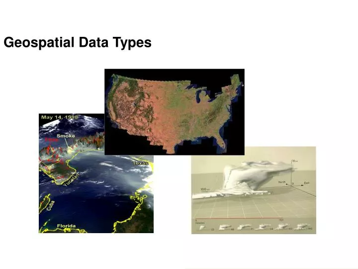
Geospatial Data Types. Data Types. Two general views to organizing spatial data: Objects Monitoring measurement points, rivers, structures Have attributes or features attached to them Point, line or area format Values exist at entity locations

E N D
Data Types • Two general views to organizing spatial data: • Objects • Monitoring measurement points, rivers, structures • Have attributes or features attached to them • Point, line or area format • Values exist at entity locations • Commonly stored and rendered in raster format (grids) • Fields • Continuous data such as temperature gradient fields and satellite imagery • Values exist over an area • Every location has a value • Commonly stored and rendered in raster format (grids)
Raster and Vector Data Models Real World 600 1 2 3 4 5 6 7 8 9 10 G 1 B Trees 500 2 G B G 3 B 400 G G 4 B Trees Y-AXIS 5 B G G 300 B BK 6 G G House 7 B 200 B B 8 River 100 9 B 200 500 100 300 600 400 10 B X-AXIS Raster Representation Vector Representation adapted from Lembo, 2003
Advantages Good representation of reality Relatively compact data structure Accurate graphics Disadvantages Complex data structures Some spatial analysis is difficult or impossible to perform Vector – Advantages and Disadvantages
Raster – Advantages and Disadvantages • Advantages • Simple data structure • Uniform size and shape • Computationally cheaper to process • Disadvantages • Large amount of data • Less visually pleasing (“blocky”) • May lose information due to generalization • Projection transformation is difficult • Different scales between grids can make comparison difficult
Objects and Fields Objects and fields can be transformed to the other type Objects Vectors Fields Raster adapted from Bolstad, 2002
Vector vs. Raster Burroughs, 1996
5 6 7 8 10 13 5 7 8 10 12 13 4 5 12 8 15 (16-20) 15 3 4 (11-15) 5 13 15 16 3 5 (6-10) 17 15 11 14 (1-5) 4 5 2 17 16 16 Landcover Raster Grid Legend Mixed conifer Douglas fir Oak savannah Grassland
5 6 7 8 10 13 5 7 8 10 12 13 4 5 12 8 15 15 3 4 5 13 15 16 3 5 17 15 11 14 4 5 2 17 16 16 Raster = Grid Matrix of Equal-Area Cells Pixel columns Abbreviation for PICTURE ELEMENT, which is the smallest unit in an image. In raster based GIS systems, attribute information can be assigned to each pixel. rows The bounding box defines the geographic extent of the grid in terms of its coordinates [min_x, max_x, min_y, max_y]
5 6 7 8 10 13 5 7 8 10 12 13 4 5 12 8 15 15 3 4 5 13 15 16 3 5 17 15 11 14 4 5 2 17 16 16 Grid File Format (ASCII) ncols 6 nrows 6 xllcorner 210 yllcorner 370 cellsize 20 nodata_value 0 5, 6, 7, 8, 10, 13 5, 7, 8, 10, 12, 13 4, 5, 8, 12, 15, 15 3, 4, 5, 13, 15, 16 3, 5, 11, 14, 15, 17 2, 4, 5, 16, 16, 17
5 6 7 8 10 13 5 7 8 10 12 13 4 5 12 8 15 15 3 4 5 13 15 16 3 5 17 15 11 14 4 5 2 17 16 16 Contoured Plots Also known as an Isopleth Plot
Map Scale • Map scale is based on the representative fraction, the ratio of a distance on the map to the same distance on the ground. • Most maps used in GIS fall between 1:1 million and 1:1000. • A GIS is scaleless because maps can be enlarged and reduced and plotted at many scales other than that of the original data. • To meaningfully compare maps in a GIS, both maps MUST be at the same scale
Scale of a baseball earth • Baseball circumference = 226 mm • Earth circumference approx 40 million meters • Scale is 1:177 million
Scale Dependent Measurements How long is Maine’s coastline? length=340 km length=355 km length=415 km From Longley et al., 2001
Resolution 25 meter 5 meter Same number of pixels (rows and columns) 1 meter
Resolution 1 meter 5 meter 25 meter Same geographic area (m X m)
Spatial Dimensionality Another way to classify spatial object types is by their dimensionality 0-dimensional, L0 points and nodes 1-dimensional, L1 lines 2-dimensional, L2 (x,y) areas, polygons 3-dimensional, L3 (x, y, z) volumes 4-dimensional, L4 (x, y, z, t) 3-D plus time
Attributes Attributes are the values and properties of an object or entity
Types of Attributes A common approach to classifying attributes is based on their level of measurement • Nominal– Simply identifies or classifies an entity so that it can be distinguished from another. e.g. sensor ID, building name • Cannot be manipulated using mathematical operations. However, frequency distributions are meaningful. • Ordinal – Values based on an order or ranking, e.g. agricultural potential classes • Cannot be manipulated using mathematical operations. However, frequency distributions are meaningful. • Interval – Differences between entities are defined using fixed equal units, e.g. Celsius temperature • Can be manipulated using addition and subtraction • Ratio - Differences between entities can be defined using ratios, e.g. distance • Can be manipulated using multiplication and division • Cyclic - differences between entities depending on repeating sequence, e.g. wind direction
Structured Query Language (SQL) SQL is a formal search language that allows you to work with, access and filter data stored in a relational database format The most common use for SQL is to retrieve subsets of data based on specified conditions SELECT column name FROM data table name WHERE data condition
ArcGIS Select by Attribute SELECT * FROM MO_STN WHERE O3 > 80 AND PM25 > 15
Classification Schemas Natural breaks: classes are defined according to apparently natural groupings of data values. (GIS programs that automatically determine classes usually base them on relatively large jumps in data values.) Quantile breaks: classes are defined by having an equal number of observations Equal interval breaks: classes are defined by uniform intervals Standard deviation breaks: classes are defined by differences from the mean value.
Color Brewer http://www.personal.psu.edu/faculty/c/a/cab38/ColorBrewerBeta.html
Summary • Two general data types: object & field • Generally, “handled” as either vector or raster • Data can have multiple attributes (properties) associated with features or grid cells • Levels of measurement helps formalize the arithmetic and statistics that are appropriate for a particular dataset
Gistutorial\UnitedStates States Counties Cities Capitals Utah Nevada Pennsylvania Gistutorial\Layers Tutorial3-1.mxd Tutorial3-NativeAmericans.mxd