Download
1 / 50
750 likes | 1.58k Views
Chapter 5 Public Goods. Reading. Essential reading Hindriks, J and G.D. Myles Intermediate Public Economics. (Cambridge: MIT Press, 2005) Chapter 5. Further reading

E N D
Chapter 5 Public Goods
Reading • Essential reading • Hindriks, J and G.D. Myles Intermediate Public Economics. (Cambridge: MIT Press, 2005) Chapter 5. • Further reading • Andreoni, J. ‘Impure altruism and donations to public goods: a theory of warm-glow giving’, Economic Journal (1990) 100: 464—477. • Abrams, B.A. and M.A Schmitz ‘The crowding out effect of government transfers on private charitable contributions: cross sectional evidence’, National Tax Journal (1984) 37: 563—568. • Bergstrom, T.C., L. Blume, L. and H. Varian ‘On the private provision of public goods’, Journal of Public Economics (1986) 29: 25—49. • Bohm, P. ‘Estimating demand for public goods: an experiment’, European Economic Review (1972), 3: 55—66. • Cornes, R.C. and T. Sandler The Theory of Externalities, Public Goods and Club Goods. (Cambridge: Cambridge University Press, 1996) [ISBN 0521477182 hcr] Chapters 6–10.
Reading • Cullis, J. and P. Jones Public Finance and Public Choice, (Oxford: Oxford University Press, 1998) [ISBN 0198775792 pbk] Chapter 3. • Isaac, R.M., K.F. McCue and C.R Plott ‘Public goods in an experimental environment’, Journal of Public Economics (1985), 26: 51—74. • Itaya, J.-I., D. de Meza and G.D. Myles ‘In praise of inequality: public good provision and income distribution’, Economics Letters (1997), 57: 289—296. • Oakland, W.H. ‘Theory of public goods’ in A.J. Auerbach and M. Feldstein (eds.), Handbook of Public Economics (Amsterdam: North-Holland, 1987) [ISBN 044487612X hbk]. • Samuelson, P.A. ‘The pure theory of public expenditure’, Review of Economics and Statistics (1954) 36: 387—389. • Warr, P.G. ‘The private provision of a pure public good is independent of the distribution of income’, Economics Letters (1983) 13: 207—211. • Challenging reading • Groves, T. and J. Ledyard ‘Optimal allocation of public goods: a solution to the ‘free rider’ problem’, Econometrica (1977) 45: 783—809.
Reading • Itaya, J.-I., D. de Meza and G.D. Myles ‘Income distribution, taxation and the private provision of public goods’, Journal of Public Economic Theory (2002) 4: 273—297. • Foley, D.K. ‘Lindahl’s solution and the core of an economy with public goods’, Econometrica (1970) 38: 66—72. • Laffont, J.-J. ‘Incentives and the allocation of public goods’, in A.J. Auerbach and M. Feldstein (eds.), Handbook of Public Economics. (Amsterdam: North-Holland, 1987) [ISBN 044487612X hbk]. • Milleron, J.-C. ‘Theory of value with public goods: a survey article’, Journal of Economic Theory (1972) 5: 419—477.
Introduction • National defense: all inhabitants are simultaneously protected • Radio broadcast: received simultaneously by all listeners in range of the transmitter • These are both public goods • If many consumers benefit from a single unit of provision the efficiency theorems do not apply
Definitions • A pure public good satisfies: • Nonexcludability If the public good is supplied, no consumer can be excluded from consuming it • Nonrivalry Consumption of the public good by one consumer does not reduce the quantity available for consumption by any other • A private good is excludable at no cost and is perfectly rivalrous
Goods can possess different combinations of rivalry and excludability Club goods are studied in chapter 6 Common property resources are studied in chapter 7 These are both examples of impure public goods Definitions Figure 5.1: Typology of goods
Private Provision • Each consumer has an incentive to rely on others to provide the public good • The reliance on others is called free-riding • This leads to inefficiency since too little public good is provided • All consumers will benefit from providing more public good
Private Provision • Consider two consumers who allocate their incomes between a private good and a public good • The consumers take prices as fixed • Each consumer derives a benefit from the provision of the other • This introduces strategic interaction into the decision processes • The Nash equilibrium has to be found
Private Provision • Let be the provision of consumer h • Fig. 5.1 shows the preferences of consumer 1 • Assume consumer 2 provides • The utility of consumer 1 is maximized at • Varying traces out the locus of choices for consumer 1 Figure 5.2: Preferences and choice
Private Provision • Fig. 5.2 constructs the locus of choice for consumer 2 • If consumer 1 chooses to provide consumer 2 chooses • The locus of chooses is given by the solid line • This is the best-response function Figure 5.3: Best reaction for 2
Private Provision • The Nash equilibrium is where the choices of the two consumers are the best reactions to each other • Neither has an incentive to change their choice • This occurs at a point where the best-response functions cross • The equilibrium choices are and Figure 5.4: Nash equilibrium
The private provision equilibrium is inefficient But it is privately rational A simultaneous increase in provision by both consumers gives a Pareto improvement Pareto-efficient allocations are points of tangency between indifference curves Private Provision Figure 5.5: Inefficiency of equilibrium
Efficient Provision • At a Pareto-efficient allocation the indifference curves are tangential • This does not imply equality of the marginal rates of substitution because the indifference curves are defined over quantities of the public good purchased by the two consumers • Instead the efficiency condition involves the sum of marginal rates of substitution and is termed the Samuelson rule
Efficient Provision • The tangency condition is • Calculating the derivatives • The marginal rate of substitution is
Efficient Provision • The tangency condition then becomes • This is the Samuelson rule • The sum of marginal rates of substitution is equated to the marginal rate of transformation between public and private goods • The marginal rate of substitution measures the marginal benefit to a consumer of another unit of public good • The marginal rate of transformation is the marginal cost of another unit
Efficient Provision • For two private goods the efficiency condition is • Why the difference? • An additional unit of a private good goes to either consumer 1 or consumer 2 • Efficiency is achieved when both place the same marginal value upon it • An additional unit of public good benefits both consumers • The marginal benefits are therefore summed
Allocation through Voting • The level of public good provision is frequently determined by voting • Political parties promise different levels of provision • Majority voting determines which party wins • Need to assess whether this attains efficiency
Allocation through Voting • There is a population of H voters • The cost of the public good is shared equally • Consumer h has income • The utility function is • Each consumer votes for the value of G that maximizes utility
Allocation through Voting • Rank the consumers by income so • Fig. 5.5 shows that the preferred levels of public good satisfy • Assume an odd number of voters • The median voter will be decisive • Their choice will win the vote Figure 5.6: Allocation through voting
Allocation through Voting • The choice of the median voter satisfies • The necessary condition can be written as • So voting achieves efficiency only if
Allocation through Voting • Can any prediction be made? • Income has a long right tail • If MRS falls with income the median MRS is greater than mean • This implies voting results in Gm exceeding the efficient level • There is no guarantee that voting will achieve efficiency
Personalized Prices • With private goods consumption is adjusted to equate marginal valuation with market price • With public goods it is not possible for consumers to adjust consumption • This suggests adjusting prices to match the valuations of the fixed quantity • This is the basis of personalized pricing Table 5.1: Prices and quantities
Personalized Pricing • Personalized pricing can be achieved by setting the share of the public good financed by each consumer • The Lindahl mechanism asks each consumer to announce public good demand as a function of share • The shares are adjusted until all consumers demand the same quantity • If the demands honestly reflect preferences the equilibrium is efficient
Personalized Pricing • The tax shares for the two consumers are t1 and t2 • The shares satisfy t1+t2= 1 • The budget constraint of h is xh + thGh = Mh • Gh is chosen to maximize utility • Equilibrium shares ensure G1=G2=G* • Efficiency is achieved Figure 5.7: Lindahl equilibrium
Personalized Pricing • The choice problem is • This has necessary condition • Summing over consumers • The allocation satisfies the Samuelson rule
Personalized Pricing • Personalized pricing suffers from two significant drawbacks • There are practical difficulties of implementation when there are many consumers • The Lindahl mechanism is not incentive compatible and consumers have an incentive to announce false demand functions
Personalized Pricing • Assume consumer 1 is honest • If consumer 2 were also honest the equilibrium would be eL • The equilibrium can be moved to eM if consumer 2 announces a false demand function • Allocation eM maximizes the utility of consumer 2 given the demand function of consumer 1 Figure 5.8: Gaining by false announcement
Mechanism Design • Consumers will make false announcements if this is advantageous • This will distort the outcome • Mechanism design is the search for allocation mechanisms that cannot be manipulated • A preference revelation mechanism ensures true preferences are revealed
Mechanism Design • Understatement • The benefit of the public good is vh = 1 • Cost of 1 is met by those reporting rh= 1 • Announcements either rh= 0 or rh= 1 • Provided if r1+r2≥ 1 • Nash equilibrium is rh= 0, h = 1, 2 • No provision Figure 5.9: Announcements and payoffs
Mechanism Design • Overstatement • Benefit of the public good is v1 = 0, v2 = ¾ • Cost of 1 is shared equally • Reports are r1 = 0 or 1, r2 = ¾ or 1 • Provide if r1+r2≥ 1 • Equilibrium r1= 0, r2= 1 • Inefficient provision Figure 5.10: Payoffs and overstatement
Mechanism Design • The Clarke-Groves mechanism ensures • True values are revealed • The public good is provided only when it should be • The allocation of cost is taken as given • Consumers report their net benefits (benefit – cost) • Public good is provided if sum of net benefits is positive
Mechanism Design • If the public good is provided side payments are made • These side payments reflect the fact that extracting the truth is costly • The side payments internalize the net benefit of the public good to other players
Mechanism Design • Net benefits are vh = -1 or vh = 1 (the mechanism must work for both) • Reports are rh = -1 or rh = 1 • The public good is provided if r1+r2≥ 0 • If provided the payoffs are v1 + r2 for player 1 and v2 + r1for player 2 • The rh in the payoffs are the side payments Figure 5.11: Clarke-Groves Mechanism
Mechanism Design Figure 5.12: Payoffs for Player 1 • When v1 = -1 a truthful report is weakly dominant for player 1 • When v1 = 1 player 1 is indifferent between truth and false statement • The mechanism ensures there is no incentive not to be truthful
Mechanism Design • The mechanism ensures truthful reports and efficient provision of the public good • The drawback is the cost of the side payments • If v1 = v2 =1 the total cost of the side payments is 2 • The side payments must be financed from outside the mechanism
More on Private Provision • The private provision model predicts inefficiency • The model also makes additional predictions that can be contrasted to evidence • These predictions also have implications for government policy
More on Private Provision • Consider a transfer of D from consumer 1 to consumer 2 • The transfer shifts the indifference curves from the solid to the dashed • The point delivers the same utilities after the transfer as the point did before • The best response function also shifts Figure 5.13: Effect of income transfer
More on Private Provision • Consumer 1 reduces contribution to the public good by D • Consumer 2 raises contribution by D • Total public good provision remains at • Consumption of private good does not change • The equilibrium is invariant to the transfer Figure 5.14: New equilibrium
More on Private Provision • Assume H identical consumers • Let be provision of all consumers but one • Symmetry of equilibrium implies • As H increases the equilibrium moves up the reaction function • The contribution of each individual tends to zero Figure 5.15: Additional consumers
More on Private Provision • The predictions of the model have been tested using experiments • The typical experiment gives participants a fixed income to spend • Income can be divided between a public good and a private good • The private good has higher private benefit and the public good a higher social benefit
More on Private Provision • Fig. 5.16 shows typical payoffs • It is individually rational to spend all income on the private good • It is socially optimal to spend all income on the public good • The Nash equilibrium of the one-shot game has no investment in the public good Figure 5.16: Public good experiment
More on Private Provision • In experiments average contribution to the public good is 30 to 90 percent of income • Most observations fall in the 40 to 50 percent range • Among students the contribution to the public good is lowest for economists and falls with number of year of economics • Repeating the game results in lower contributions in later rounds
More on Private Provision • A number of explanations have been proposed for these results • The players may not use non-Nash conjectures. This response has the problem of being arbitrary • Consumers may derive a warm glow from making a contribution. The warm glow raises the benefit and so raises contribution • Social interaction can be admitted. This could be a social custom or a consideration of fairness
Fund-Raising Campaigns • The model used so far has a single round of voluntary contributions • If consumers observe the equilibrium is inefficient they may wish to have a second round of contribution • The same logic can be applied repeatedly suggesting efficiency may be approached afer numerous rounds • This logic is now assessed using a fund-raising game
Fund-Raising Campaigns • In the fund-raising game a target level of funds must be achieved before a public good can be provided • The game has an infinite horizon • The target for funds is C • There are two identical players (X and Y) who derive benefit B from the public good • The good is socially desirable with B < C < 2B • Both players have discount rate d for delaying completion for one period • The players alternate in making contributions
Fund-Raising Campaigns • In a contribution campaign the contributions are paid at the time they are made • This form of campaign is used if no credible commitment can be made • Assume it is now the turn of X to make a contribution at time T • The maximal contribution X will make to finish the campaign is xT = [1 – d]B • At T – 1 the maximum contribution Y will make (knowing X will finish the campaign at T) is yT–1= d[1 – d2]B • This reasoning can be continued back in time
Fund-Raising Campaigns • This process is shown in Fig. 5.17 • Summing these contributions gives [1 – d]B + d[1 – d2]B + d3[1 – d2]B + …= B • The total contributions never exceed the individual valuation • The contribution campaign will never finance the public good Figure 5.17: A contribution campaign
Fund-Raising Campaigns • In the subscription campaign donation pledges are made • Contributions are only made when and if pledges are sufficient to finance the public good • This alters the strategic structure and the amount raised is equal to the total valuation of the contributors • Start at time T with X about to make a pledge • The maximum X will pledge to finish the campaign is xT = [1 – d]B
Fund-Raising Campaigns • The maximum that Y will pledge at T – 1 knowing that X will complete the campaign is yT–1= [1 – d2]B • Summing these pledges gives [1 – d]B + [1 – d2]B + d[1 – d2]B + …= 2B • It is therefore possible to fund the project because C < 2B • This result shows that allowing contributions to be repeated may remove the inefficiency but requires the ability to make binding commitments