Download
1 / 16
160 likes | 311 Views
Equilibrium in a Simple Model. Equilibrium. Key concept in economics illustrate with the simplest possible macro model Equilibrium is a point of balance or stability Specifically in economics it is a point where economic agents plans are mutually consistently and therefore are realised

E N D
Equilibrium • Key concept in economics • illustrate with the simplest possible macro model • Equilibrium is a point of balance or stability • Specifically in economics it is a point where economic agents plans are mutually consistently and therefore are realised • Disequilibrium • plans are inconsistent • then someone’s plans are not realised • Somebody is disappointed • Behaviour will change • The economy will change • so not stable or balanced
MACROECONOMIC EQUILIBRIUM • First, Output (which equals Income) is a function of inputs: for simplicity, Capital (K) and Labour (L) Y = f(K, L) • This is the amount firms planto spend • There will also be Aggregate Demand (Ep) • the amount of Expenditure which agents plan to make • Agents: Households, firms, the Government and foreigners • In equilibrium plans are consistent Y = Ep • Later we will see that sometimes Output or Income do not equal planned expenditure: this corresponds to a disequilibrium • The general idea is that in equilibrium the forces acting on some variable (Y) are balanced and hence Y will not change.
AGGREGATE EXPENDITURE • Conventionally we look at separate components of aggregate (planned) expenditure: C, I, G, NX. This is because they behave differently. • Crucially C (Consumption) depends partly on Income: so part of Expenditure depends on Income: hence the term Induced (Consumption) Expenditure • Other components of Expenditure are Autonomous: this should be understood as depending on something other than Income. • We have • an Autonomous component of Consumption (Ca) • Investment (Ip) • Government purchases (G) • Foreign demand (NX)
THE CONSUMPTION FUNCTION (1) • An equation that describes consumption plans • Very Generally, Consumption depends on Disposable Income (Y minus net taxes, T). • More specifically: C = Ca + c(Y – T) • the “Autonomous” and “Induced” elements are on the right-hand side. • The coefficient c (The Marginal Propensity to Consume) is > 0 and < 1, implying that for any given increase or decrease in disposable income C will change in the same direction, but by a lesser amount. • i.e. 0 < dC/d(Y – T) = c < 1 • This is a model of consumption insofar as it is a simplified representation of how people make their consumption plans • It doesn’t say that plans will be successful • It is very simple (even simplistic): no interest rates, future income, life cycle
THE CONSUMPTION FUNCTION (2) • Note: Ca is “Autonomous” consumption; C/Y (APC) falls as Y increases; c (MPC) is < APC. C 45 (C = Y) Ca + c(Y – T) Slope = c Ca 0 (Y-T )
CONSUMPTION AND SAVINGS • We have Y = C + S + T: hence S = Y – C – T • Which gives: S = Y – Ca – cY + cT – T • S = – Ca + Y(1 – c) – T(1– c) • S = – Ca + (1 – c)(Y – T) • And the MPS = dS/dY = (1 – c)d(Y – T) • Suppose Y = 500, Ca = 50, c = 0.8, T = 150: Find C, S. • C = 50 + 0.8(500 -150) = 50 + 0.8(350) = 330 • S = – 50 + 0.2(350) = 20 • Suppose Y increases to 600: (Y – T) increases to 450 • dC/d(Y – T) = 0.8, so C increases to 410 • dS/d(Y– T) = 0.2 so S increases to 40
EQUILIBRIUM • As always equilibrium is plans are consistent • Specifically in this case planned production is equal to planed demand Y = Ep, • Sub in equation for planned expenditure (“Aggregate Demand”) Ep= C + Ip + G + NX • To get Y = C + Ip + G + NX • Sub in consumption function • To get: Y= Ca + cY – cT + Ip + G + NX • Note • cYis the one part of Expenditure which depends on Income • The other components (Ca –cT + Ip + G + NX) may be termed autonomous planned spending, in that they do not depend in Income (at least for now…) • Alternatively we might term them the Endogenous and Exogenous components of planned spending.
Eqmvs Identity • We have an accounting identity: Y = C + I + G + NX • This different from the equilibrium condition • The equilibrium condition describes planned magnitudes • These plans may or may not be realised • The identity describes what actually happens • This may or may not have been what was planned • Thus the equilibrium condition is true only for certain values of the variables • The identity is true always • Best thought of as an account rule
DISEQUILIBRIUM • To illustrate the concept of equilibrium consider a numerical example • Suppose we have Ca = 50, c = 0.8, T = 150, Ip = 40, G = 150, NX = 60 • Suppose we have Y = 600 • Is Income at equilibrium? • Calculate Planned expenditure (Aggregate Demand) • Ep= Ca + c(Y – T) + Ip + G + NX • = 50 + 0.8(450) + 40 + 150 + 60 • 300 + 360 = 660 • So Planned Production (Y) < Planned Expenditure (Ep) • Somebody’s plans will not be realised • Production is not sufficient to meet demand • Plans must be updated • How? • We will assume that production will be increased to meet demand • Note we assume prices don’t change • Will provide empirical evidence later
EQUILIBRIUM • What is Equilibrium Y in this case? • We could try by trial and error • Or we could solve the equations • By definition equilibrium is where planned production equals planned expenditure: Y = Ep Y = Ca + c(Y – T) + Ip + G + NX Y – cY = Ca – cT + Ip + G + NX Y(1-c) = Ca – cT + Ip + G + NX Y(1 – c) = Ap • Where Ap = Autonomous planned spending = Ca – cT + Ip + G + NX • Plug in numbers • Y = Ap/(1 –c) = (50-120+40+150+60)/(0.2) = 180/0.2 = 900 • One can re-check by plugging in all the components of Ep when Y = 900 and getting Ep = 900, i.e. equilibrium
EQUILIBRIUM • This can all be illustrated graphically • When Ep > Y, Y < Ye hence Y rises: similarly when Ep < Y….. Ep 45 (Èp = Y) Ep = Ap + c(Y – T) Ap 0 Y Ye
Comment • The process is self sustaining • If we are not at equilibrium there is an automatic adjustment process that will bring us into equilibrium • If this were not the case no point in studying eqm • If not at eqm we are heading there • We assume for the moment that the adjustment process works by producers changing out put to meet demand • We also assume that prices don't change • Seems counter intuitive • This model effectively assumes that prices are fixed • Will provide empirical evidence alter that this is approximately true in the short run
A CHANGE IN AGGREGATE SPENDING (1) • Suppose Ip and therefore Ap fall by 40, Ye1 falls to Ye2 by a multiple of 40 (Ye > Ap) Ep 45 (Èp = Y) Ep1 = Ap1 + c(Y – T) Ep2 = Ap2 + c(Y – T) Ap1 Ap2 0 Y Ye2 Ye1
A CHANGE IN AGGREGATE SPENDING (2) • Initial Equilibrium is: Y1 = Ap1 + c(Y1 – T) • Following Shock to Ap: Y2 = Ap2 + c(Y2 – T) • Subtracting: Y2 – Y1 = Ap2 – Ap1 + c(Y2 – Y1) • i.e. Y =Ap + c Y • so Y(1 – c) = Ap • And thus: Y/Ap = 1/(1 – c) or 1/s • So if c = 0.8, s = 0.2, multiplier = 5: etc…. • Intuitively: an increase in Ap (say G) is spent: it becomes income to someone who re-spends c times the increase, etc… • Y = G(1 + c + c2 + c3 + ….. + cn) • cY = G(c c2 c3 + ….. + cn+1) then adding • And Y(1 c) =G(1) (the other terms cancel) • So Y/G = 1/(1-c) or 1/s
CHANGES IN SAVINGS, TAXES • In the previous example, an increase in G of 100 produced an increase of 500 in Y. • As T is given this means that (Y – T) increased by 500, and C increased by c.Y so savings increased by s.Y = 100 • Financing the increased G by selling Bonds to Savers?? • Now what happens if T were reduced by 100 instead of increasing G? • Initial Equilibrium is: Y1 = Ap + c(Y1 – T1) • Following cut in T: Y2 = Ap + c(Y2 – T2) • i.e. Y =c.Y– c.T • So Y(1 – c) = – c.T • Y/ T = – c/(1 – c) • Thus if c = 0.2, –c/(1 – c) = – 0.8/0.2 = – 4. • Note sign, magnitude (intuition of this)