Download
1 / 56
560 likes | 875 Views
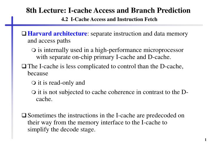
8th Lecture: I-cache Access and Branch Prediction 4.2 I-Cache Access and Instruction Fetch. Harvard architecture : separate instruction and data memory and access paths is internally used in a high-performance microprocessor with separate on-chip primary I-cache and D-cache.

E N D
8th Lecture: I-cache Access and Branch Prediction4.2 I-Cache Access and Instruction Fetch • Harvard architecture: separate instruction and data memory and access paths • is internally used in a high-performance microprocessor with separate on-chip primary I-cache and D-cache. • The I-cache is less complicated to control than the D-cache, because • it is read-only and • it is not subjected to cache coherence in contrast to the D-cache. • Sometimes the instructions in the I-cache are predecoded on their way from the memory interface to the I-cache to simplify the decode stage.
Instruction Fetch • The main problem of instruction fetching is control transfer performed by jump, branch, call, return, and interrupt instructions: • If the starting PC address is not the address of the cache line, then fewer instructions than the fetch width are returned. • Instructions after a control transfer instruction are invalidated. • A multiple cache lines fetch from different locations may be needed in future very wide-issue processors where often more than one branch will be contained in a single contiguous fetch block. • Problem with target instruction addresses that are not aligned to the cache line addresses: • Self-aligned instruction cache reads and concatenates two consecutive lines within one cycle to be able to always return the full fetch bandwidth. Implementation: • either by use of a dual-port I-cache, • by performing two separate cache accesses in a single cycle, • or by a two-banked I-cache (preferred).
Prefetching and Instruction Fetch Prediction • Prefetching improves the instruction fetch performance, but fetching is still limited because instructions after a control transfer must be invalidated. • Instruction fetch prediction helps to determine the next instructions to be fetched from the memory subsystem. • Instruction fetch prediction is applied in conjunction with branch prediction.
4.3 Branch Prediction • Branch prediction foretells the outcome of conditional branch instructions. • Excellent branch handling techniques are essential for today's and for future microprocessors. • The task of high performance branch handling consists of the following requirements: • an early determination of the branch outcome (the so-called branch resolution), • buffering of the branch target address in a BTAC after its first calculation and an immediate reload of the PC after a BTAC match, • an excellent branch predictor (i.e. branch prediction technique) and speculative execution mechanism, • often another branch is predicted while a previous branch is still unresolved, so the processor must be able to pursue two or more speculation levels, • and an efficient rerolling mechanism when a branch is mispredicted (minimizing the branch misprediction penalty).
Misprediction Penalty • The performance of branch prediction depends on the prediction accuracy and the cost of misprediction. • Prediction accuracy can be improved by inventing better branch predictors. • Misprediction penalty depends on many organizational features: • the pipeline length (favoring shorter pipelines over longer pipelines), • the overall organization of the pipeline, • the fact if misspeculated instructions can be removed from internal buffers, or have to be executed and can only be removed in the retire stage, • the number of speculative instructions in the instruction window or the reorder buffer. Typically only a limited number of instructions can be removed each cycle. • Rerolling when a branch is mispredicted is expensive: • 4 to 9 cycles in the Alpha 21264, • 11 or more cycles in the Pentium II.
4.3.1 Branch-Target Buffer or Branch-Target Address Cache • The Branch Target Buffer (BTB) or Branch-Target Address Cache (BTAC) stores branch and jump target addresses. • It should be known already in the IF stage whether the as-yet-undecoded instruction is a jump or branch. • The BTB is accessed during the IF stage. • The BTB consists of a table with branch addresses, the corresponding target addresses, and prediction information. • Variations: Branch Target Cache (BTC): stores one or more target instructions additionally.Return Address Stack (RAS): a small stack of return addresses for procedure calls and returns is used additional to and independent of a BTB.
Prediction Branch address Target address bits ... ... ... Branch-Target Buffer or Branch-Target Address Cache
4.3.2 Static Branch Prediction • Static Branch Prediction predicts always the same direction for the same branch during the whole program execution. • It comprises hardware-fixed prediction and compiler-directed prediction. • Simple hardware-fixed direction mechanisms can be: • Predict always not taken • Predict always taken • Backward branch predict taken, forward branch predict not taken • Sometimes a bit in the branch opcode allows the compiler to decide the prediction direction.
4.3.3 Dynamic Branch Prediction • In a dynamic branch prediction scheme the hardware influences the prediction while execution proceeds. • Prediction is decided on the computation history of the program. • After a start-up phase of the program execution, where a static branch prediction might be effective, the history information is gathered and dynamic branch prediction gets effective. • In general, dynamic branch prediction gives better results than static branch prediction, but at the cost of increased hardware complexity.
T NT Predict Not Predict Taken Taken T NT One-bit Predictor
One-bit vs. Two-bit Predictors • A one-bit predictor correctly predicts a branch at the end of a loop iteration, as long as the loop does not exit. • In nested loops, a one-bit prediction scheme will cause two mispredictions for the inner loop: • One at the end of the loop, when the iteration exits the loop instead of looping again, and • one when executing the first loop iteration, when it predicts exit instead of looping. • Such a double misprediction in nested loops is avoided by a two-bit predictor scheme. • Two-bit Prediction: A prediction must miss twice before it is changed when a two-bit prediction scheme is applied.
T NT NT NT (11) (10) (01) (00) Predict Strongly Predict Weakly Predict Weakly Predict Strongly Taken Taken Not Taken Not Taken T T T NT Two-bit Predictors(Saturation Counter Scheme)
NT T NT NT (11) (10) (01) (00) Predict Strongly Predict Weakly Predict Weakly Predict Strongly Taken Taken Not Taken Not Taken T T NT T Two-bit Predictors(Hysteresis Scheme)
Two-bit Predictors • The two-bit prediction scheme is extendable to an n-bit scheme. • Studies showed that a two-bit prediction scheme does almost as well as an n-bit scheme with n>2. • Two-bit predictors can be implemented in the Branch Target Buffer (BTB) assigning two state bits to each entry in the BTB. • Another solution is to use a BTB for target addresses and a separate Branch History Table (BHT) as prediction buffer. • A mispredict in the BHT occurs due to two reasons: • either a wrong guess for that branch, • or the branch history of a wrong branch is used because the table is indexed. • In an indexed table lookup part of the instruction address is used as index to identify a table entry.
Two-bit Predictors and Correlation-based Prediction • Two-bit predictors work well for programs which contain many frequently executed loop-control branches (floating-point intensive programs). • Shortcomings arise from dependent (correlated) branches, which are frequent in integer-dominated programs. Example:if (d==0) /* branch b1*/ d=1; if (d==1) /*branch b2 */ ...
if (d==0) /* branch b1*/ d=1; if (d==1) /*branch b2 */ ... Example: bnez R1,L1 ; branch b1 (d0) addi R1, R0,#1 ; d==0, so d=1 L1: subi R3, R1,#1 bnez R3, L2 ; branch b2 (d 0) ... L2: ... • Consider a sequence where d alternates between 0 and 2 a sequence of NT-T-NT-T-NT-T for branches b1 and b2 • The execution behavior is given in the following table: ? ?
One-bit predictor initialized to “predict taken” bnez R1,L1 ; branch b1 (d0) addi R1, R0,#1 ; d==0, so d=1 L1: subi R3, R1,#1 bnez R3, L2 ; branch b2 (d 0) ... L2: ... d alternates between 0 and 2 Initial prediction T T d==0 d==2 d==0 b1: b2: NT NT T T NT NT
T NT NT NT (11) (10) (01) (00) Predict Strongly Predict Weakly Predict Weakly Predict Strongly Taken Taken Not Taken Not Taken T T T NT Two-bit saturation counter predictor initialized to “predict weakly taken” bnez R1,L1 ; branch b1 (d0) addi R1, R0,#1 ; d==0, so d=1 L1: subi R3, R1,#1 bnez R3, L2 ; branch b2 (d 0) ... L2: ... d alternates between 0 and 2 Initial prediction WT WT d==0 d==2 d==0 b1: b2: WNT WNT WT WT WNT WNT
NT T NT NT (11) (10) (01) (00) Predict Strongly Predict Weakly Predict Weakly Predict Strongly Taken Taken Not Taken Not Taken T T NT T Two-bit predictor (Hysteresis counter) initialized to “predict weakly taken” bnez R1,L1 ; branch b1 (d0) addi R1, R0,#1 ; d==0, so d=1 L1: subi R3, R1,#1 bnez R3, L2 ; branch b2 (d 0) ... L2: ... d alternates between 0 and 2 Initial prediction WT WT d==0 d==2 d==0 b1: b2: SNT SNT WNT WNT SNT SNT
Predictor Behavior in Example • A one-bit predictor initialized to “ predict taken” for branches b1 and b2, every branch is mispredicted. • A two-bit predictor of of saturation counter scheme starting from the state “predict weakly taken” every branch is mispredicted. • The two-bit predictor of UltraSPARC mispredicts every second branch execution of b1 and b2. • A (1,1) correlating predictor takes advantage of the correlation of the two branches; it mispredicts only in the first iteration when d = 2.
Correlation-based Predictor • The two-bit predictor scheme uses only the recent behavior of a single branch to predict the future of that branch. • Correlations between different branch instructions are not taken into account. • The correlation-based predictors or correlating predictors are branch predictors that additionally use the behavior of other branches to make a prediction. • While two-bit predictors use self-history only, the correlating predictor uses neighbor history additionally. • Notation: (m,n)-correlation-based predictor or (m,n)-predictor uses the behavior of the last m branches to choose from 2m branch predictors, each of which is a n-bit predictor for a single branch. • Branch history register (BHR): The global history of the most recent m branches can be recorded in a m-bit shift register where each bit records whether the branch was taken or not taken.
Pattern History Tables PHTs (2-bit predictors) Branch address ... ... ... ... 10 1 1 ... ... ... ... select Branch History Register BHR 1 0 (2-bit shift register) Correlation-based Prediction(2,2)-predictor
Prediction behavior of (1,1) correlating predictor bnez R1,L1 ; branch b1 (d0) addi R1, R0,#1 ; d==0, so d=1 L1: subi R3, R1,#1 bnez R3, L2 ; branch b2 (d 0) ... L2: ... d alternates between 0 and 2 b1 b2 1 1 0: 1: 1 BHR PHT 1 1 Initial prediction T T d==0 b1: b2:
Prediction behavior of (1,1) correlating predictor bnez R1,L1 ; branch b1 (d0) addi R1, R0,#1 ; d==0, so d=1 L1: subi R3, R1,#1 bnez R3, L2 ; branch b2 (d 0) ... L2: ... d alternates between 0 and 2 b1 b2 1 1 0: 1: 0 BHR PHT 0 1 Initial prediction T T d==0 b1: b2: NT
Prediction behavior of (1,1) correlating predictor bnez R1,L1 ; branch b1 (d0) addi R1, R0,#1 ; d==0, so d=1 L1: subi R3, R1,#1 bnez R3, L2 ; branch b2 (d 0) ... L2: ... d alternates between 0 and 2 b1 b2 1 0 0: 1: 0 BHR PHT 0 1 Initial prediction T T d==0 d==2 b1: b2: NT NT
Prediction behavior of (1,1) correlating predictor bnez R1,L1 ; branch b1 (d0) addi R1, R0,#1 ; d==0, so d=1 L1: subi R3, R1,#1 bnez R3, L2 ; branch b2 (d 0) ... L2: ... d alternates between 0 and 2 b1 b2 1 0 0: 1: 1 BHR PHT 0 1 Initial prediction T T d==0 d==2 b1: b2: NT NT T
Prediction behavior of (1,1) correlating predictor bnez R1,L1 ; branch b1 (d0) addi R1, R0,#1 ; d==0, so d=1 L1: subi R3, R1,#1 bnez R3, L2 ; branch b2 (d 0) ... L2: ... d alternates between 0 and 2 b1 b2 1 0 0: 1: 1 BHR PHT 0 1 Initial prediction T T d==0 d==2 b1: b2: NT NT T T
Two-level Adaptive Predictors • Developed by Yeh and Patt at the same time (1992) as the correlation-based prediction scheme. • The basic two-level predictor uses a single global branch history register (BHR) of k bits to index in a pattern history table (PHT) of 2-bit counters. • Global history schemes correspond to correlation-based predictor schemes. • Denotation: GAg: • a single global BHR (denoted G) and • a single global PHT (denoted g), • A stands for adaptive. • All PHT implementations of Yeh and Patt use 2-bit predictors. • GAg-predictor with a 4-bit BHR length is denoted as GAg(4).
shift direction Branch Pattern Branch History Table History 1 1 0 0 (PHT) ... Register (BHR) predict: 1100 1 1 taken Index ... Implementation of a GAg(4)-predictor • In the GAg predictor schemes the PHT lookup depends entirely on the bit pattern in the BHR and is completely independent of the branch address.
Mispredictions can be restrained by additionally using: • the full branch address to distinguish multiple PHTs (called per-address PHTs), • a subset of branches (e.g. n bits of the branch address) to distinguish multiple PHTs (called per-set PHTs), • the full branch address to distinguish multiple BHRs (called per-address BHRs), • a subset of branches to distinguish multiple BHRs (called per-set BHRs), • or a combination scheme.
Branch address Per-address PHTs BHR ... ... ... ... 1 1 0 0 ... 1 1 Index ... ... ... Implementation of a GAp(4) predictor • Gap(4) means a 4-bit BHR • a PHT for each branch.
n bits of branch address Per-set PHTs n BHR ... ... ... ... 1 1 0 0 ... 1 1 Index ... ... ... GAs(4, 2n) • Gas(4,2n) means a 4-bit BHR • n bits of the branch address are used to choose among 2n PHTs with 24 entries each.
Compare Correlation-based (2,2)-predictor (left) with Two-level Adaptive GAs(4,2n) predictor (right) n bits of branch address Pattern History Tables PHTs (2-bit predictors) Per-set PHTs n Branch address BHR ... ... ... ... ... ... ... ... 1 1 0 0 10 ... 1 1 1 1 Index ... ... ... ... ... ... ... select Branch History Register BHR 1 0 (2-bit shift register)
Two-level Adaptive Predictors:Per-address history schemes • The first-level branch history refers to the last k occurrences of the same branch instruction (using self-history only!) • Therefore a BHR is associated with each branch instruction. • The per-address branch history registers are combined in a table that is called per-address branch history table (PBHT). • In the simplest per address history scheme, the BHRs index into a single global PHT. denoted as PAg (multiple per-address indexed BHRs, and a single global PHT).
Per-address PHT BHT ... ... Branch address 1 1 0 0 Branch address 1 1 1 1 0 0 Index ... ... Pag(4)
b1 b2 Per-address Per-address PHTs BHT ... ... Branch address b1 ... ... 1 1 0 0 ... Branch address b2 1 1 1 1 0 0 0 1 Index ... ... ... ... Pap(4)
Two-level Adaptive Predictors: Per-set history schemes • Per-set history schemes (SAg, SAs, and SAp): the first-level branch history means the last k occurrences of the branch instructions from the same subset. Each BHR is associated with a set of branches. • Possible Set attributes: • branch opcode, • the branch class assigned by the compiler, or • the branch address (most important!).
Per-set PHT BHT ... ... n n bits of 1 1 0 0 branch address n n bits of 1 1 1 1 0 0 branch address Index ... ... Sag(4)
Sas(4) b1, b2 Per-set BHT Per-set PHTs n n bits of branch address b1 ... ... ... ... n ... n n bits of branch address b2 1 1 1 1 0 0 Index ... ... ... ...
Two-level Adaptive Predictors Full table: single global PHT per-set PHTs per-address PHTs single global BHR GAg GAs GAp per-address BHT PAg PAs PAp per-set BHT SAg SAs SAp
Estimation of hardware costs In the table b is the number of PHTs or entries in the BHT for the per-address schemes. P and s denotes the number of PHTs or entries in the BHT for the per-set schemes.
Two-level Adaptive Predictors(Simulations of Yeh and Patt using the SPEC89 benchmarks) • The performance of the global history schemes is sensitive to the branch history length. • Interference of different branches that are mapped to the same pattern history table is decreased by lengthening the global BHR. • Similarly adding PHTs reduces the possibility of pattern history interference by mapping interfering branches into different tables. • Global history schemes are better than the per-address schemes for the integer SPEC89 programs, • utilize branch correlation, which is often the case in the frequent if-then-else statements in integer programs • Per-address schemes are better for the floating-point intensive programs. • better in predicting loop-control branches which are frequent in the floating-point SPEC89 benchmark programs. • The per-set history schemes are in between both other schemes.
gselect and gshare Predictors • gselect predictor: concatenates some lower order bit of the branch address and the global history • gshare predictor: uses the bitwise exclusive OR of part of the branch address and the global history as hash function. • McFarling: gshare slightly better than gselect Branch Address BHR gselect4/4 gshare8/8 00000000 00000001 00000001 00000001 00000000 00000000 00000000 00000000 11111111 00000000 11110000 11111111 11111111 10000000 11110000 01111111 In book mistakenly 1!
Hybrid Predictors • The second strategy of McFarling is to combine multiple separate branch predictors, each tuned to a different class of branches. • Two or more predictors and a predictor selection mechanism are necessary in a combining or hybrid predictor. • McFarling: combination of two-bit predictor and gshare two-level adaptive, • Young and Smith: a compiler-based static branch prediction with a two-level adaptive type, • and many more combinations! • Hybrid predictors often better than single-type predictors.
Simulations of Grunwald 1998 Table 1.1. SAg, gshare and MCFarling‘s combining predictor
Results • Simulation of Keeton et al. 1998 using an OLTP (online transaction workload) on a PentiumPro multiprocessor reported a misprediction rate of 14% with an branch instruction frequency of about 21%. • The speculative execution factor, given by the number of instructions decoded divided by the number of instructions committed, is 1.4 for the database programs. • Two different conclusions may be drawn from these simulation results: • Branch predictors should be further improved • and/or branch prediction is only effective if the branch is predictable. • If a branch outcome is dependent on irregular data inputs, the branch often shows an irregular behavior. Question: Confidence of a branch prediction?
4.3.4 Predicated Instructions and Multipath Execution- Confidence Estimation • Confidence estimation is a technique for assessing the quality of a particular prediction. • Applied to branch prediction, a confidence estimator attempts to assess the prediction made by a branch predictor. • A low confidence branch is a branch which frequently changes its branch direction in an irregular way making its outcome hard to predict or even unpredictable. • Four classes possible: • correctly predicted with high confidence C(HC), • correctly predicted with low confidence C(LC), • incorrectly predicted with high confidence I(HC), and • incorrectly predicted with low confidence I(LC).
Implementation of a confidence estimator • Information from the branch prediction tables is used: • Use of saturation counter information to construct a confidence estimator speculate more aggressively when the confidence level is higher • Used of a miss distance counter table (MDC): Each time a branch is predicted, the value in the MDC is compared to a threshold. If the value is above the threshold, then the branch is considered to have high confidence, and low confidence otherwise. • A small number of branch history patterns typically leads to correct predictions in a PAs predictor scheme. The confidence estimator assigned high confidence to a fixed set of patterns and low confidence to all others. • Confidence estimation can be used for speculation control,thread switching in multithreaded processors or multipath execution
Predicated Instructions • Provide predicated or conditional instructions and one or more predicate registers. • Predicated instructions use a predicate register as additional input operand. • The Boolean result of a condition testing is recorded in a (one-bit) predicate register. • Predicated instructions are fetched, decoded and placed in the instruction window like non predicated instructions. • It is dependent on the processor architecture, how far a predicated instruction proceeds speculatively in the pipeline before its predication is resolved: • A predicated instruction executes only if its predicate is true, otherwise the instruction is discarded. In this case predicated instructions are not executed before the predicate is resolved. • Alternatively, as reported for Intel's IA64 ISA, the predicated instruction may be executed, but commits only if the predicate is true, otherwise the result is discarded.
Predication Example if (x = = 0) { /*branch b1 */ a = b + c; d = e - f; } g = h * i; /* instruction independent of branch b1 */ (Pred = (x = = 0) ) /* branch b1: Pred is set to true in x equals 0 */ if Predthena = b + c; /* The operations are only performed */ ifPredthene = e - f; /* if Pred is set to true */ g = h * i;