Download
1 / 27
360 likes | 1.6k Views
Stock Returns Predictability using Markov Regime Switching Model. Gheorghe Marius Bogdan. Paper Objectives. To analyze the process of estimation of the Markov regime switching models in stock returns

E N D
Stock Returns Predictability using Markov Regime Switching Model Gheorghe Marius Bogdan
Paper Objectives • To analyze the process of estimation of the Markov regime switching models in stock returns • To make a short comparison between the results obtained using a Present Value Model based on the available data in the Romanian stock market (Betfi Index) and a model using a Markov Regime Switching process
MRS – First definition of the concept • The first concept about MRS date to at least R. E. Quandt and J. M. Henderson (1958) in their work “Microeconomic Theory: A Mathematical Approach” • After 15 years later, Quandt together with Goldfeld (1973) introduced a particularly useful version of these models, referred to in the following papers as a Markov-switching model
MRS – Hamilton work • Hamilton (1989) applied this technique to the study of post-war business cycles in the United States, where he studied regime shifts from positive to negative growth rates in real GNP • Hamilton(1989) extended Markov regime-switching models to the case of autocorrelated dependent data. This seminal paper has prompted many subsequent analyses investigating some sort of Markov regime change in an empirical model • Hamilton found the Markov regime shift approach to be an objective criterion for defining and measuring economic recessions. • Hamilton and Lin (1996) also report that economic recessions are a main factor in explaining conditionally switching moments of financial distributions.
MRS – Basic components • We have an unobservable variable in the time series that switches between a certain number of states and for each state we have an independent price process • We have a probability law that governs the transition from one state to another • Markov switching model is achieved by considering joint conditional probability of each of future states as a function of the joint conditional probabilities of current states and the transition probabilities • The conditional probabilities of current states are input, passing through or being filtered by the transition probability matrix, to produce the conditional probabilities of futures states as output
MRS – Basic Benefits • effectively deal with modeling financial time series that are affected by time-varying properties • ease by which they can deal with the stochastic properties that underlie most financial and economic data, whether it be for equity, fixed income or derivatives • Conventional framework with a fixed density function or a single set of parameters may not be suitable and it is necessary to include possible structural changes, market jumps or craches in the analysis • Provide flexible features that might include mean reversion, asymmetric distributions and the time varying nature of a distribution of moments
MRS – business cycle approach • economic relationship behind financial market movements – that being the business cycle • Cecchetti, Lam and Schaller (1999) show how dividend payments affect stock return distributions due to changes in economic growth • Hamilton and Lin (1996) also report that economic recessions are a main factor in explaining conditionally switching moments of financial distributions • Campbell, Lettau, Malkiel and Xu (2001) and Schwert (1989) have also shown that there is a counter cyclical effect of economic activity upon stock volatility • Ebell (2001) also shows the relationship between the business cycle and return distributions
MRS - non-linear behavior of exchange trading • Speculative trading is common among financial markets and this can lead to fads and bubbles • Flood and Hodrick (1990) indicates this may suggest evidence of mis-specified fundamentals within financial prices • Funk, Hall and Sola(1994), Hamilton (1989) and van Norden and Schaller (1999) show that this type of behavior can easily be modeled using application of MRS models • Dewachter (2001), applied for speculative regime shifts when examining foreign exchange trading – the proof that Markov models can be suitable for most financial markets
MRS – Present applicability • The actual methodology utilised to incorporate Markov regime switching models is varied • Many models are switching regressions with latent state variables, in which parameters move discretely between a fixed number of regimes, with the switching controlled by an unobservable state variable • The primary study dates back to Hamilton’s (1989) work on simple mean switching, which has led to a number of extensions that are used • Turner,Startz and Nelson’s (1989) model allows for variations in both the first and second moments of a distribution between regimes • Hamilton and Susmel(1994) examines a conditional heteroscedastic Markov regime switching model • now a wide range of alternative models deal with varying distribution dynamics and asymmetries - Ang and Bekaert (2002), Ang and Chen (2002)
MRS - Hamilton approach (multi-state) • Hamilton confines his analysis to the cases where the density function of Yt depends only on finitely many past values of st : • for some finite integer m, and the corresponding conditional likelihood is P(st,st-1, . . . , st-m| Yt-1), he starts with the assumption that st follows a first-order Markov chain: • where , which is called the transition probability, is specified as a constant coefficient that is independent of time t (time-invariant) • st : regime indicator which cannot be observed, st = 1, …, J
MRS - Hamilton approach • The conditional likelihood P (st , . . . , st-m| Yt-1) can then be calculated iteratively through two equations as follows:
MRS - Hamilton approach • The term P (st-1, . . . , st-m-1| Yt-1), in which the first st-1 term and Yt-1are both subscripted by the same period of time, is then computed as follows: for t = 1, 2, . . . , T . Given initial values P (s1, sо, s-1, . . . , s-(m-1)| Yо), we can calculate by iteration.
MRS - Filtering • Having P (st,st-1, . . . , st-m| Yt), we can eliminate the st,st-1, . . . , st-m terms as follows: This is called the filtering probability. Basing on observation it can “filter out” the unobserved state of world.
MRS - Predicting • In the same way, we can also calculate all the predicting probability.The probability becomes predicting probability as we restrict r < t. • For instance, the one-step ahead predicting probability can be calculated by “integrating out” the st, st-1, . . . , st-m terms in :
MRS - Smoothing • On the other hand, when r > t, we can have the so-called smoothed probability This is for retrieving all the past states of the world. For example, for j = 1, 2, …, m, can be easily calculated as :
MRS - Smoothing • A special smoothed probability which is based on all T observations of yt, can be calculated as (Hamilton, 1989) : Where:
MRS – Data • data used for analyze is the BetFi index from the Bucharest Stock Exchange (BSE) at weekly frequency beginning with the starting date of this index (november 2000 ) and ending with end of june 2008 • I also used for analyze a subsample from 2005 until 2008 to be able to catch the variability and the structure switching of the returns
MRS – The Matlab Program • The developed Matlab program is very flexible and the central point of this flexibility resides in the input argument S, which controls for where to include markov switching effect. • For instance, if you have 2 explanatory variables ( x1t , x2t ) and if the input argument S, which is passed to the fitting function MS_Regress_Fit.m, is equal to S=[1 1], then the model for the mean equation is: Where: represents the state at time t, that is, St = 1 … K , where K is the number of states is the model’s standard deviation at state St is the beta coefficient for explanatory variable i at state St where i goes from 1 to n is the residue which follows a particular distribution (in this case Normal or Student)
MRS – results table • Period 2000 – 2008 : • Period 2005 – 2008 :
Present Value Model - Data • the returns used in the model estimation are constructed at trimester frequency beginning with 2000:02 and ending with 2007:04 as follows: • BetFi returns – taking into account that this index has components formed by 5 financial investments companies and the starting date of existing was november 2000, I estimate the returns from the period april 2000 until november 2000, folowing the structure of this index; Source: BSE • Short rate returns – I calculate the short rate return, following the formula: (Bubid+Bubor)/2, where Bubid and Bubor were considered on a horizon of 3 months; Source: National Bank of Romania (NBR) • Dividendreturns – I calculate the dividend on index following the structure and the percentage of the each company in the index. To obtain trimester data, i interpolate the values between two consecutive years. The type of the function that I used for interpolation is cubic spline data interpolation ; Source: BSE • Consumer Price Index – source: National Institute of Statistics
Present Value Model - Comments • The statistical significance of the return forecast is marginal, with a t-statistic only a little above two • presents regressions of the real and excess value-weighted stock return on its dividend-price ratio, in annual data • The 4–7% R2 do not look that impressive, but the R2 rises with horizon • The slope coefficient of over three in the • top two rows means that when dividend yields rise one percentage point, prices rise another two percentage points on average • all variation in market price-dividend ratios corresponds to changes in expected excess returns—risk premiums—and none corresponds to news about future dividend growth