Download
1 / 8
130 likes | 529 Views
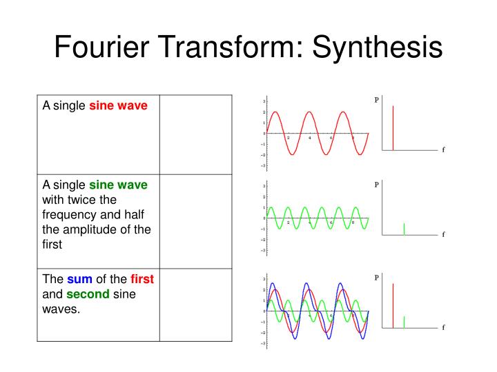
Fourier Transform: Synthesis. Fourier Transform. Y = fft(y,512); Pyy = Y.* conj(Y) / 512; f = 1000*(0:256)/512; plot(f,Pyy(1:257)) title('Frequency content of y') xlabel('frequency (Hz)'). t = 0:0.001:0.6; x = sin(2*pi*50*t)+sin(2*pi*120*t); y = x + 2*randn(size(t));

E N D
Fourier Transform Y = fft(y,512); Pyy = Y.* conj(Y) / 512; f = 1000*(0:256)/512; plot(f,Pyy(1:257)) title('Frequency content of y') xlabel('frequency (Hz)') t = 0:0.001:0.6; x = sin(2*pi*50*t)+sin(2*pi*120*t); y = x + 2*randn(size(t)); plot(1000*t(1:50),y(1:50)) title('Signal Corrupted with Zero-Mean Random Noise') xlabel('time (milliseconds)') fft example from Matlab documentation
Fourier Transform 1/f^1, “pink” noise versus 1/f^0 “white” noise
Fourier Transform Neural oscillations are patterened, relate to each other, **but NOT by an integer ratio**
Fourier Transform • Power at some frequencies depends on behavioral state. (note: here, power is whitened)
Fourier Transform Deviations from 1/f in time are significant…see self-criticality
Fast Fourier Transform Y = fft(y,512); Pyy = Y.* conj(Y) / 512; f = 1000*(0:256)/512; plot(f,Pyy(1:257)) title('Frequency content of y') xlabel('frequency (Hz)') t = 0:0.001:0.6; x = sin(2*pi*50*t)+sin(2*pi*120*t); y = x + 2*randn(size(t)); plot(1000*t(1:50),y(1:50)) title('Signal Corrupted with Zero-Mean Random Noise') xlabel('time (milliseconds)') What is a Spectrogram? fft example from Matlab documentation
Power Spectra • Example of fast-Fourier with small temporal windows over long behavioural epochs (p. 106) • Example of Fourier averaged over 1s time window (plot on left) and smoothed using smaller, overlapping windows to reveal dynamics (main plot) fixation period face on