Data assimilation for systems with multiple time-scales

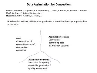
1. Data assimilation for systems with multiple time-scales Mike Cullen and Gordon Inverarity 4 September 2007

2. Introduction

3. Motivation Data assimilation optimised for short-range (12 to 36 hour) operational forecasts in the extratropics. Same techniques must be applicable globally, though maybe non-optimal in the tropics Convective-scale data assimilation for shorter timescales will require different techniques.

4. Observed behaviour of the system Forecasting for timescales of 12-36 hrs in the extratropics requires accurate prediction of weather systems. These are characterised by timescales greater than 1/f, where f is the Coriolis parameter expressing the Earth’s rotation. This corresponds to fluid trajectories taking more than a day to change direction by π/2. The atmosphere contains many other motions with faster timescales.

5. Implications for data assimilation The observation network is designed to measure the geostrophic disturbances, it is not really sufficient even for this task. Most other types of motion can only be properly observed during special field campagns. It is important to use the observations to define the geostrophic disturbances properly.

6. Basic 4D-Var

7. The problem Given a previous forecast which takes the form of a trajectory calculated using an (imperfect) numerical model. This is called the background trajectory. Given a new set of (imperfect) observations. Constrain the forecast trajectory using the new observations and the background trajectory to give the best possible new forecast.

8. 4D-Var

9. 4D-Var

10. 4D-Var

11. What is 4D-Var? I Assume a nonlinear forecast model Mi,i-1 and uncorrelated zero-mean Gaussian model error Wi with covariance Q

12. What is 4D-Var? II Assume a nonlinear observation operator Hi and uncorrelated zero-mean Gaussian observation error Vi with covariance R

13. 4D-Var with model error Huge minimisation state vector

14. 4D-Var with a perfect forecast model Smaller minimisation state vector

15. Effect of perfect model formulation I The observations are fitted using a model trajectory. The trajectory is defined by its initial values, which are now the only control parameters. The error in the background trajectory , in reality a mixture of model error and errors in previous observations, is assumed to be solely due to errors in observations. The resulting analysis trajectory is

16. Effect of perfect model formulation II This solution is statistically optimal if: • The model is perfect • Perturbations to the model trajectory evolve according to linear dynamics • The error in the initial value is Gaussian with zero mean All these assumptions are seriously deficient in a real situation

17. Alternative formulation

18. Alternative formulation Wish to acknowledge imperfect model, without losing requirement to fit observations with a model trajectory, thus ensuring consistency with forecast.

19. Distributed-background 4D-Var Penalise the difference between the background and analysis trajectories throughout the assimilation window Reduces to traditional 4D-Var when a=p/n, the Jacobian can accurately evolve increments and These are the assumptions listed earlier.

20. Exploitation Can now use different growth assumption based on diagnostics Expect that non-geostrophic errors are ‘permanently saturated’. Thus the flow consists of geostrophic disturbances, the errors in which grow in time, and a background of other motions whose total energy is constant in time. This would lead to no growth of errors in non-geostrophic motions in the assimilation window. Will show that this discourages fitting of observations with such motions.

21. Diagnostic evidence of error growth

22. Evaluation of assumptions We can examine the linear growth assumption by comparing the difference of two nonlinear runs with the evolution of a linearised perturbation model. Many of the physical processes represented in the model are highly nonlinear-limiting the accuracy demonstrated by such a test.

23. Linearisation test over 6 hour period Relative error

24. Singular vectors Even using a linear model, the growth of perturbations is not simply exponential or wave-like because of the time-dependent trajectory about which the evolution is linearised. Thus the growth has to be assessed over a given time interval. A particular choice of perturbation is referred to as a ‘singular vector’.

25. Behaviour of standard 4D-Var If observations late in 4D-Var window, they will be fitted using the most rapidly growing singular vectors, since that gives the smallest penalty in the initial value. The growth is assessed over the assimilation window, typically 6-12 hours. x x x x x * Background

26. Error growth In the real system, error growth in the rotationally dominated (geostrophic) disturbances saturates at a point when the weather systems are completely out of phase. This takes a time of order 2 weeks. The errors in other motions saturate at a much lower value and on a shorter timescale (~ 1 day).

27. Singular vector growth Singular vector calculations by Corinna Klapproth and Tim Payne using operational data from July 2003 follow. They show that the most rapid growth is in non-geostrophic modes unless the period over which the growth is calculated is greater than 36 hrs. This is much longer than an assimilation window, so 4D-Var will tend to use other types of perturbation to fit the observations..

28. Energy partition in geostrophic and ageostrophic

29. Energy partition in geostrophic and ageostrophic

30. Energy partition in geostrophic and ageostrophic

31. Energy partition in geostrophic and ageostrophic

32. Energy partition in geostrophic and ageostrophic

33. Energy partition in geostrophic and ageostrophic

34. Error growth due to imperfect model The combination of the growth of differences between the truth ‘model’ and the forecast model and the growth of perturbations under the action of the forecast model can be inferred using verification figures from operational forecasts. These suggest a linear growth (greater in first 24 hrs). The same is true for errors in significant weather systems, such as tropical and extratropical cyclones.

35. Error growth in key parameters Rms errors in surface pressure (thick solid), 500 hpa height (dashed) and 200 hpa wind (thin solid) over N hemisphere in 1995

36. Illustration using toy model

37. 3-body problem: Inverarity (2007) 12-dimensional Hamiltonian problem of a sun-planet-moon orbital system with fast and slow timescales Nonlinear 4D-Var using Gauss-Newton method to solve grad J = 0 Explicit symplectic integrator with analytical Jacobian B matrix generated using an extended Kalman filter (model error variance tuned to ensure sensible filter behaviour)

38. Multiple timescales Slow timescale associated with planet’s orbit round sun (7200 timesteps) Fast timescale with moon’s orbit round planet (540 timesteps) Choose assimilation period of about 50% of moon’s orbital period (corresponds to 6 hr period in real system)

39. 3-body orbits – Watkinson (2006)

40. Sun mass = 1.0 Planet mass = 0.1 Moon mass = 0.01 Sun mass = 1.0 Planet mass = 0.1 Moon mass = 0.011 Perfect (truth) vs imperfect (forecast) model

41. Issues to study A systematically imperfect model does not satisfy the assumptions of 4D-Var. The growth of differences between the truth model and the forecast model may dominate the growth of perturbations under the action of the forecast model. The linear model used to describe error growth in the forecast model is not adequate.

42. Model error growth Time unit 1000 timesteps

43. Linearisation tests Show evolution of differences from nonlinear runs compared with growth of difference predicted by linear model. Linear assumption good for sun’s position/momentum (slow dynamics); not for moon’s position/momentum (fast dynamics) as desired to match real system

44. Test results-(forecast model)

45. Assimilation test Use standard 4D-Var with B derived from extended Kalman filter, would be ‘correct’ if model was perfect stochastic model. Run further 300 steps after EKF ‘analysis’ to get background state. Complete set of observations during assimilation window. Also use distributed background term with two ‘nodes’, B for both taken as time average from EKF.

46. Results with no assimilation-900 steps Position Momentum Red=Sun, Blue=Planet Green=Moon

47. Results with standard 4D-Var-900 steps Position Momentum Red=Sun, Blue=Planet Green=Moon

48. Results with distributed Jb-900 steps Position Momentum Red=Sun, Blue=Planet Green=Moon

49. Results with no assimilation-4000 steps Position Momentum Red=Sun, Blue=Planet Green=Moon

50. Results with standard 4D-Var-4000 steps Position Momentum Red=Sun, Blue=Planet Green=Moon