Download
1 / 7
90 likes | 375 Views
Cooled by LN 2. Amplifier:. ADC. Memory. CCD Detectors. CCD=“charge coupled device” Silicon semiconductor chip array of up to crossed electrodes -> potential wells current models: up to 2048x2048 wells trap photoelectrons Readout method:

E N D
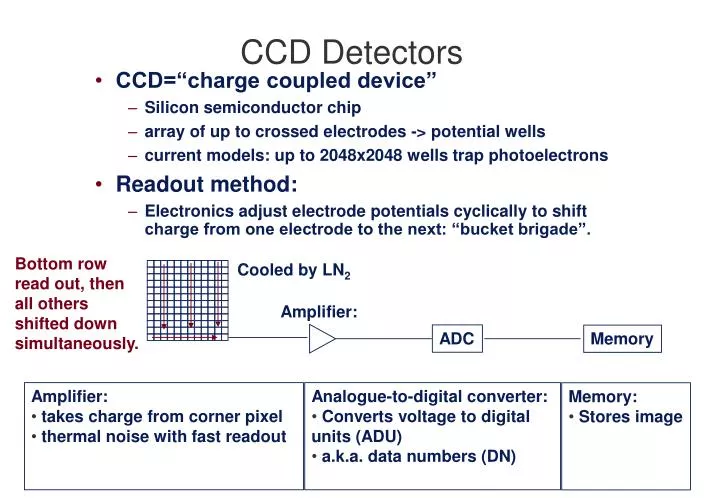
Cooled by LN2 Amplifier: ADC Memory CCD Detectors • CCD=“charge coupled device” • Silicon semiconductor chip • array of up to crossed electrodes -> potential wells • current models: up to 2048x2048 wells trap photoelectrons • Readout method: • Electronics adjust electrode potentials cyclically to shift charge from one electrode to the next: “bucket brigade”. Bottom row read out, then all others shifted down simultaneously. • Amplifier: • takes charge from corner pixel • thermal noise with fast readout • Analogue-to-digital converter: • Converts voltage to digital units (ADU) • a.k.a. data numbers (DN) • Memory: • Stores image
The pros and cons of CCDs • Advantages: • Quantum efficiency (QE) ~ 80 % (400 nm - 1 m) • Linearity to (better than) << 0.1 % • Dynamic range: Pixel well depth ~ 106 e–, RMS readout noise ~ 4 to 10 e– • Fixed format pixel grid • Can extend blue response (thinned back-illuminated chip or coronene coating) • Disadvantages: • Readout noise 4 to 10 e– RMS • Slow readout ≥ 10 to 100 s • Cosmic-ray hits limit exposure times • Saturation via wells filling up and limited ADC range • Charge “bleeding” down columns, then across rows • Blemishes (charge traps, hot pixels) • Gaps between pixels
CCD calibration Raw image • Two main steps: • bias subtraction • flat-field division • “Flat-field frame”: • Measures pixel-to-pixel • sensitivity variations under • uniform illumination. • “Bias frame” = zero-exposure image • Measures constant signal added by • readout electronics
Measuring bias and readout noise • Calibrate by taking mean or median of many zero-exposure images and/or • “Overscan” the CCD by reading out additional rows of data for which no physical pixels exist. • Cosmic ray hits must be removed, e.g. by taking median of many frames. • “Readout noise” = (Bxy): • Voltage drift may cause <Bxy> to vary in time: • Need to scale bias frame to match overscan.
Flat-field division • Direct imaging: • twilight sky or inside of telescope dome • OR median of many dark sky frames of different fields (median eliminates stars) • Spectroscopy: • spectrum of internal comtinuum source (tungsten lamp) • Pixel-to-pixel sensitivity variations => Fxy is never uniform, even with uniform illumination. • Take 10 to 30 flats with high exposure levels • subtract bias form each • scale to common mean value (if lamp/sky brightness drifts) • take average or median (to reject cosmic-ray hits) • fit a polynomial to flat field and divide so that <Fxy> ~ 1. This preserves data numbers/photons while correcting pixel-to-pixel variations.
Measuring the gain of a CCD -- 1 • The gain of a CCD is the number of photo- electrons per ADU (DN). • Let X be a random variable representing number of ADU recorded in a pixel. • There are 3 types of noise that contribute to variance 2(X) • Readout noise 2 • Poisson noise :number of photons detected = X / G • “Scale noise” with variance f2X2 -- usually dealt with by flat-fielding • At low count-rates, readout noise (=constant) dominates. • At high count-rates, Poisson noise ~X1/2 dominates.
Measuring the gain of a CCD -- 2 • Take several flats with different levels of illumination. • Divide into sub-areas and measure <X>,2(X) locally • Make log-log scatterplot of (X) vs. <X>: • Determine values of (0,G) that give best-fitting curve of form: G=1 G=3.2 G=10 slope=1/2 4.2 In this illustrative case we find readout noise = 4.2 DN and gain G = 3.2 electrons per DN