Download
1 / 15
200 likes | 575 Views
Continuous Probability Distributions. Many continuous probability distributions, including: Uniform Normal Gamma Exponential Chi-Squared Lognormal Weibull. Standard Normal Distribution. Table A.3: “Areas Under the Normal Curve”. Applications of the Normal Distribution.

E N D
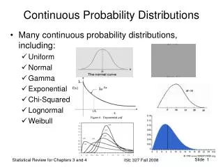
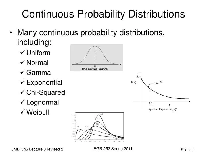
Continuous Probability Distributions • Many continuous probability distributions, including: • Uniform • Normal • Gamma • Exponential • Chi-Squared • Lognormal • Weibull EGR 252 Spring 2011
Standard Normal Distribution • Table A.3: “Areas Under the Normal Curve” EGR 252 Spring 2011
Applications of the Normal Distribution • A certain machine makes electrical resistors having a mean resistance of 40 ohms and a standard deviation of 2 ohms. What percentage of the resistors will have a resistance less than 44 ohms? • Solution: Xis normally distributed with μ = 40 and σ= 2 and x = 44 P(X<44) = P(Z< +2.0) = 0.9772 Therefore, we conclude that 97.72% will have a resistance less than 44 ohms. What percentage will have a resistance greater than 44 ohms? EGR 252 Spring 2011
The Normal Distribution “In Reverse” • Example: Given a normal distribution with = 40 and σ = 6, find the value of X for which 45% of the area under the normal curve is to the left of X. • Solution: If P(Z < k) = 0.45, what is the value of k? 45% of area under curve less than k k = -0.125 from table in back of book Z = (x- μ) / σ Z = -0.125 = (x-40) / 6 X = 39.25 Z values 39.25 40 X values EGR 252 Spring 2011
Normal Approximation to the Binomial • If n is large and p is not close to 0 or 1, or if n is smaller but p is close to 0.5, then the binomial distribution can be approximated by the normal distribution using the transformation: • NOTE: When we apply the theorem, we apply a continuity correction: add or subtract 0.5 from xto be sure the value of interest is included (drawing a picture helps you determine whether to add or subtract) • To find the area under the normal curve to the left of x+ 0.5, use: EGR 252 Spring 2011
Look at example 6.15, pg. 191-192 The probability that a patient recovers is p = 0.4 If 100 people have the disease, what is the probability that less than 30 survive? n = 100 μ= np =____ σ= sqrt(npq)= ____ if x = 30, then z = _____________ (Don’t forget the continuity correction.) and, P(X < 30) = P (Z < _________) = _________ (Subtract 0.5 from 30 because we are looking for P (X< x). Less than 30 for a discrete distribution is 29 or less. EGR 252 Spring 2011
The Normal Approximation: Your Turn DRAW THE PICTURE!! Using μ and σ from the previous example, 1. What is the probability that more than 50 survive? More than 50 for a discrete distribution is 51 or greater. How do we include 51 and not 50 ? Since we are looking for P (X>x) we add 0.5 to x. EGR 252 Spring 2011
The Normal Approximation: Your Turn 2 Using μ and σ from the previous example, 1. What is the probability that exactly 45 survive if we use the normal approximation to the binomial? Hint: Find the area under the curve between two values. Calculate P (X>x) by adding 0.5 to x. Calculate P (X<x) by subtracting 0.5 from x. Determine P(X=x) by calculating the difference. 2. What is the probability that exactly 45 survive if we use the binomial distribution? b(45;100,0.4) Note that n=100 is too large for the tables. Determine the value using the binomial equation. 0 …. 44 45 46 ….. 100 DRAW THE PICTURE!! EGR 252 Spring 2011
Gamma & Exponential Distributions • Sometimes we’re interested in the number of events that occur in a certain time period. • Related to the Poisson Process • Number of occurrences in a given interval or region • “Memoryless” process • Discrete • If we are interested in the time until a certain number of events occur, we will use continuous distributions (exponential and gamma). • The time until a number of Poisson events uses gamma distribution with alpha = number of events and beta = mean time. • See Examples 6.17 and 6.18 EGR 252 Spring 2011
Gamma Distribution • The density function of the random variable X with gamma distribution having parameters α (number of occurrences) and β (time or region). x > 0. μ = αβ σ2= αβ2 EGR 252 Spring 2011
Exponential Distribution • Special case of the gamma distribution with α = 1. x > 0. • Describes the time until or time between Poisson events. μ = β σ2= β2 EGR 252 Spring 2011
Is It a Poisson Process? • For homework and exams in the introductory statistics course, you will be told that the process is Poisson. • An average of 2.7 service calls per minute are received at a particular maintenance center. The calls correspond to a Poisson process. What is the probability that up to a minute will elapse before 2 calls arrive? • An average of 3.5 service calls per minute are received at a particular maintenance center. The calls correspond to a Poisson process. How long before the next call? EGR 252 Spring 2011
Poisson Example Problem 1 An average of 2.7 service calls per minute are received at a particular maintenance center. The calls correspond to a Poisson process. What is the probability that up to 1 minute will elapse before 2 calls arrive? • β = 1 / λ = 1 / 2.7 = 0.3704 • α = 2 • x = 1 What is the value of P(X ≤ 1)? Can we use a table? Must we integrate? Can we use Excel? EGR 252 Spring 2011
Poisson Example Solution Based on the Gamma Distribution An average of 2.7 service calls per minute are received at a particular maintenance center. The calls correspond to a Poisson process. What is the probability that up to 1 minute will elapse before 2 calls arrive?β = 1/ 2.7 = 0.3704 α = 2 = 0.7513 Excel = GAMMADIST (1, 2, 0.3704, TRUE) EGR 252 Spring 2011
Poisson Example Problem 2 An average of 2.7 service calls per minute are received at a particular maintenance center. The calls correspond to a Poisson process. What is the expected time before the next call arrives? α = next call =1 λ = 1/ β = 2.7 Expected value of time (Gamma) = μ= αβ Since α =1 μ = β = 1 / 2.7 = 0.3407 min. Note that when α = 1 the gamma distribution is known as the exponential distribution. EGR 252 Spring 2011